Introduction to NACA Four-Digit Airfoils
NACA four-digit airfoils are geometric representations defined primarily by two variables:
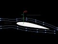
- Mean camber line: The curve representing the centerline of the airfoil, depicted in blue.
- Thickness distribution: The airfoil’s thickness above and below the mean camber line, shown as green dotted lines.
The chord length (C) is the baseline length from the leading to trailing edge, used as a reference scale.
For a foundational understanding of these concepts, see Airfoil Basics: Understanding Shape, Terminology, and NACA Naming.
Understanding NACA Four-Digit Notation
A typical NACA designation, such as NACA 2412, encodes:
- m (max camber): Maximum camber as a percentage of chord length (e.g., 2% for 2412).
- p (position of max camber): Location of max camber along the chord as a fraction of chord length (e.g., 0.4 for 2412 means 40% from leading edge).
- t (thickness): Maximum thickness as a percentage of chord (e.g., 12% for 2412).
Defining the Mean Camber Line
The mean camber line is defined by two piecewise functions depending on the chordwise position relative to p:
- From leading edge (0) to p: [ y_c = \frac{m}{p^2} (2px - x^2) ]
- From p to trailing edge: [ y_c = \frac{m}{(1-p)^2} ((1 - 2p) + 2px - x^2) ]
If m and p are zero, the airfoil is symmetric with a flat mean camber line.
Calculating the Camber Line Derivative
The slope ( \frac{dy_c}{dx} ) of the mean camber line is:
- For ( x < p ): [ \frac{dy_c}{dx} = \frac{2m}{p^2} (p - x) ]
- For ( x \geq p ): [ \frac{dy_c}{dx} = \frac{2m}{(1-p)^2} (p - x) ]
This slope helps determine the angle (( \theta )) of the camber line tangent:
[ \theta = \arctan \left( \frac{dy_c}{dx} \right) ]
To deepen your understanding of related geometric considerations, review Introduction to Shape Analysis and Applied Geometry in 6838 Course.
Thickness Distribution Formula
The half-thickness distribution (from mean camber line to upper or lower surface) is given by:
[ y_t = 5 t \left(a_0 \sqrt{x} + a_1 x + a_2 x^2 + a_3 x^3 + a_4 x^4 \right) ]
where coefficients for a 20% thick airfoil are:
- (a_0 = 0.2969)
- (a_1 = -0.1260)
- (a_2 = -0.3516)
- (a_3 = 0.2843)
- (a_4) depends on trailing edge type (finite or sharp).
This thickness is measured perpendicular to the mean camber line.
For mathematical techniques involving curvilinear frameworks like this, see Understanding Curvilinear Coordinates: A Comprehensive Guide.
Calculating Upper and Lower Surface Coordinates
Using the camber line and thickness:
-
Upper surface coordinates: [ x_u = x - y_t \sin \theta ] [ y_u = y_c + y_t \cos \theta ]
-
Lower surface coordinates: [ x_l = x + y_t \sin \theta ] [ y_l = y_c - y_t \cos \theta ]
For symmetric airfoils (( \theta = 0 )), these simplify to vertical thickness additions above and below the chord line.
For applied calculation methods involving arc lengths and areas similar in concept to these coordinate calculations, refer to Calculating Arc Length, Triangle, and Sector Areas with Theta.
Practical Application and Upcoming Coding Tutorial
These equations provide a complete geometric description of NACA four-digit airfoils. In the next video, a MATLAB program will be developed to generate airfoil coordinates from user inputs, enabling export of data for simulations and analyses.
To connect airfoil geometry with flight mechanics practicalities, also consider Understanding Aircraft Performance: A Comprehensive Overview of Flight Mechanics.
By understanding and applying these principles, engineers and enthusiasts can accurately model NACA airfoils for aerodynamic studies and design optimization.
hey everyone in this video I'm going to be going over the nacka four-digit air foils first I'll go through uh just a
general overview of the air foils and then after that I'll go through a mathematical description of them uh in a
subsequent video I'm going to show you how to code up your own program to calculate different uh data points for
these air foils that you can export as a as a text file for use and whatever you want to do with it uh so the nacka
4digit air foil uh is a geometric description of an air foil and there are two primary variables that describe uh
the geometry of this air foil the first is the mean camber line shown in blue and you can see that here and then the
second is a thickness distribution above and below the mean camber line shown in these green dotted lines here uh my
picture is not to scale because the upper and the lower on one of these dotted lines should be equal uh C is the
cord length of the air foil I have a video on cord length that I'll post in the description uh if you want to take a
look at that and so you'll see in the literature or just in anything that you read that uh the general formula for the
air foil looks like this it's a NAA something something something something uh and you can see that it's either like
a 2412 or A2 might be something that you've that you've seen uh quite often so now let's go through what each of
these uh terms mean so the m is the maximum camber uh as percentage of the cord so in this case for the 2412 that
means that it's uh 2% so the maximum camber of the air foil the maximum camber may be like right here for this
air foil that's 2% of the cord length uh the second term is p which is the chordwise position of the maximum camber
and that for this case here it's p over 10 so this four that's not 4% that's actually 40% so that means that the
maximum camber occurs uh 4/10 of the 4/10 of the way back from the Leading Edge of the cord of the cord length so
in this case here if the maximum camber is like right about here it looks like this one might actually be five in this
in this p position and then the XX here that's one number so this 12 is one number it's not one two it's 12 and
that's the maximum section thickness uh as percentage of the cord so in this case the 12 here and the 12 here I guess
um means that it's uh has a 12% maximum thickness of the air foil as a function of the cord length the first thing we
need to do is find the mean camber line which is defined by the m and the p terms in the four-digit air foil
designation so in the npx X designation uh this is a plot of the mean camber line so without any of the thickness
applied to the air foil yet and I'm going to assume a chord length of one length unit so meter feet because we can
always multiply by a certain cord length later on so this cord length here is going to be one the Leading Edge here is
that located at x equals 0 and the trailing EDG is at x equals the chord length or one uh this P if you recall
from the previous image before uh is the location along the cord of the maximum uh camber so these are the two equations
that specify this blue line here the top one is used uh when you're going from the Leading Edge to point p and the
bottom one is used from point P to the trailing Edge uh if one thing to note is that if you have a symmetric air foil so
such as like A2 the first two numbers the m and the P are both zeros so if you look at these equations here for the uh
y coordinate the if you plug in m is equal to Z here you'll get a y-coordinate of zero uh for
both of these equations for the entire length of the of the air foil which means that for every X it'll be the y
coordinate will be at zero which means you'll just get a flat line here indicating that there's no camber so now
that we have the mean camber line equations the next thing we need to do is to find the uh derivative of the mean
camber line equations so if we have these two equations from the previous white board we just take the derivative
with respect to the x coordinate and you get these two expressions so for the front half well front up to p and then
from P to the end of the the uh cord so in this picture over here this is the main camera line I'm going to zoom in on
this little portion right here and this is the green portion here I'm going to draw take a point in black and draw a
line tangent to it and for a certain distance that we move in X along the air foil or along the cord line we need to
move a certain distance y to get to the next point and this angle here th Theta is defined as the inverse tangent of
this change in the y-coordinate over the change in the x coordinate uh which is just this equation here so the Theta you
can Define as the inverse tangent of this or this equation depending on where you are on the air foil and so the
question is why do you need to do that uh if you take this mean camber line you need to add some thickness to the air
foil and I'll go through the thickness Distribution on the next whiteboard um and you might think oh I'll just add it
vertically to the point where I'm at so if I'm add an X point along the along the air foil I'll just add the thickness
up and down but what you actually need to do is you need to add the thickness perpendicular to the mean camber line
which is where this Theta turn comes into play so once you know the slope you can uh add the thickness uh
perpendicular to this mean camber line now that we have the mean camber line which you can see in blue here we need
to add the thickness distribution to that air foil here seen in the dashed green lines uh so this is the equation
for the thickness so Y subt is a thickness distribution it's given by this equation
that has these coefficients a0 A1 A2 A3 A4 for uh each of these X terms here and
the X terms are taken into account the distance from the Leading Edge to the trailing Edge uh these coefficients are
given down here and they're defined for a 20% thickness air foil and the way that it that you can account for the
change and thickness uh given here that you defined for your air foil is this front term here which takes into account
that XX term uh the one thing to note is that this A4 coefficient here there's two of them one of them is for uh an
open trailing Edge or a finite thickness trailing Edge and another one is for a Sharp trailing Edge it's important to
note that this YT is a half thickness in the sense that it's a thickness above and a thickness below it doesn't take
into account the entire thickness so what you need to do is you need to add this thickness both above the mean
camber line perpendicular to the mean camber line and Below perpendicular to the mean camber line so now we have the
mean camber line and we also have the thickness distribution of the air foil so we can now Define the overall
coordinates of the air foil that we want to specify so here we have the mean camber line and here I have the
thickness distribution and what we're trying to find is this particular point it's a black circle and I'm calling this
one CU this is the upper surface here I'm calling this X U and Y U for the lower surface I call it x sub L and and
Y sub l so if I take this I'm going to drop a line over perpendicular to the y- AIS here like this and then you can see
it goes down to the to the point on the main cam line so I'm going to blow that up here you can see that this green line
is still the thickness distribution or Y subt and then we have this distance Alpha and the distance beta that we're
going to need to Define where this point is in space based off of the camber line and the thickness distribution so we
remember Theta from before and if we specify this distance as Alpha and that's as beta we can say from
trigonometric uh principles that the S of the Theta is equal to the alpha over YT and beta is equal to the or cosine of
theta is equal to Beta over YT and if we rearrange we get expressions for Alpha and beta in terms of YT and Theta which
we both know so we can Define points on the upper surface and the lower surface looking at the upper surface here the x
of the at a certain X distance so we're at a certain X Point here we know that the X point if it's sloping up like this
the X Point since we have to since we have to draw the uh thickness perpendicular to to the mean camber line
it's going to be less than this x point so we have this x upper is equal to the X Point minus the thickness YT time the
S of the Theta like this and it's a sign here and you might wonder oh well what happens when it's when the the trailing
Edge when it's sloping down well that is going to be even though there's a minus sign here it's going to be taken into
account in the S SN of the sin Theta term in the Y upper we're going to have y of the camber line so at a certain uh
Point here we're at a certain distance above the zero line the zero chord line already so we need to take that y of the
camber line and then we need to add the YT cos Theta or the beta distance up and this is always going to be uh positive
because on the upper surface you're always going to be adding and then similarly for the lower surface we have
the x sub l and y sub L and they're similar but they're just switched with these signs here and uh and they give
you the points that are on the bottom uh or the lower surface of the air foil there so the one thing we need to note
about these equations here is what happens when we have a symmetric air foil so when we have a symmetric air
foil uh if you recall from before or the angle Theta is going to be zero so we need to plug in the Theta is equal to Z
into these expressions and see what we get and if you do that you can see that at s of zero you get a zero so this term
goes away which means that all along the air foil you every single X point is at its actual XO which makes sense if you
look at the this is the camber line of a symmetric air foil it's a straight horizontal line if I've drawn that
correctly and that means that there's no slope so every single point that you draw
if you take this x point the thickness is going to be up a certain point at that exact X point and there's it's not
going to be moved either left or right because of the slope and now if we plug in zero to this cosine term this is a
one so we have the Y camber plus the Y thickness so the Y camber we're at this point because it's a horizontal line so
it's at zero and we need to add the thickness and we're just adding the thickness up and so it checks out that
these equations work for a symmetric air foil like A2 or whatever you want I'm going to be going over in the next video
about how to program a mat lab code that will give you uh the air foil shape based off of what you input so you can
input like a NAA 2412 or naa2 and it'll give you the coordinates for the air foil based off of how many grid points
you put in there Etc so thanks for watching
Each digit in a NACA four-digit code specifies airfoil geometry: the first digit (m) indicates maximum camber as a percentage of chord length; the second digit (p) shows the position of maximum camber as a fraction of the chord from the leading edge; and the last two digits (t) represent maximum thickness as a percentage of chord. For example, NACA 2412 has 2% maximum camber located at 40% chord length, with 12% thickness.
The mean camber line is defined by piecewise equations based on chordwise position x relative to p (position of maximum camber). For 0 ≤ x < p: y_c = (m / p²) * (2px - x²); for p ≤ x ≤ 1: y_c = (m / (1 - p)²) * ((1 - 2p) + 2px - x²). If m and p are zero, the mean camber line is flat, indicating a symmetric airfoil.
The slope dy_c/dx is derived from the mean camber line equations: for x < p, dy_c/dx = (2m / p²)(p - x); for x ≥ p, dy_c/dx = (2m / (1 - p)²)(p - x). The tangent angle θ is then θ = arctangent(dy_c/dx), which is essential for determining surface coordinates relative to the camber line.
Thickness distribution y_t (half-thickness from mean camber line) is given by y_t = 5t(a₀√x + a₁x + a₂x² + a₃x³ + a₄x⁴), where t is max thickness as a fraction of chord, and coefficients a₀ to a₄ are constants (e.g., a₀=0.2969, a₁=-0.1260). The coefficient a₄ varies with trailing edge type (finite or sharp). This formula defines thickness perpendicular to the camber line.
Using the mean camber line (y_c), thickness distribution (y_t), and camber angle θ, the surfaces are: upper surface—x_u = x - y_t sinθ, y_u = y_c + y_t cosθ; lower surface—x_l = x + y_t sinθ, y_l = y_c - y_t cosθ. For symmetric airfoils where θ=0, these simplify to adding thickness vertically above and below the chord line.
Comprehending NACA airfoil geometry enables precise modeling of airfoil shapes for aerodynamic analysis, simulation, and optimization. It allows engineers to tailor camber and thickness distributions to achieve desired lift, drag, and performance characteristics, facilitating efficient and effective aircraft or component designs.
After mastering geometric equations, a practical next step is implementing these formulas in coding environments like MATLAB to generate airfoil coordinate data programmatically. This enables easy integration into simulations, CFD analyses, and aerodynamic performance evaluations, bridging theory with real-world engineering applications.
Heads up!
This summary and transcript were automatically generated using AI with the Free YouTube Transcript Summary Tool by LunaNotes.
Generate a summary for freeRelated Summaries
Airfoil Basics: Understanding Shape, Terminology, and NACA Naming
This video covers the fundamental concepts of airfoils, including their definitions, key parts like leading and trailing edges, and how shape affects lift and drag. It also explains important terminology such as chord line and angle of attack, and breaks down the NACA airfoil naming system for better understanding of airfoil design.
Comprehensive NACA 2412 Airfoil CFD Tutorial with ANSYS Fluent
This detailed tutorial guides you through modeling, meshing, and simulating a NACA 2412 airfoil using ANSYS Fluent. Learn step-by-step how to create geometry, set mesh parameters, run simulations, and analyze lift and drag coefficients, including the impact of varying angle of attack. Practical tips on y-plus calculation and comparison with experimental data enhance your CFD skills.
Complete ANSYS Fluent Tutorial: NACA 2412 Airfoil Simulation and Analysis
Learn how to simulate the NACA 2412 airfoil in ANSYS Fluent step-by-step, from geometry creation and meshing to setting boundary conditions and performing flow analysis. This comprehensive guide includes drag and lift coefficient calculations, flow field visualization, and angle of attack effects, making it ideal for engineering students and CFD practitioners.
Understanding Aircraft Performance: A Comprehensive Overview of Flight Mechanics
This lecture delves into the intricacies of aircraft performance, focusing on flight mechanics, performance diagrams, and the calculations necessary for understanding horizontal flight. Key topics include minimum and maximum airspeed, range, endurance, and the impact of weight on performance.
Understanding Curvilinear Coordinates: A Comprehensive Guide
Dive into the world of curvilinear coordinates and their applications in engineering, physics, and mathematics.
Most Viewed Summaries

A Comprehensive Guide to Using Stable Diffusion Forge UI
Explore the Stable Diffusion Forge UI, customizable settings, models, and more to enhance your image generation experience.

Kolonyalismo at Imperyalismo: Ang Kasaysayan ng Pagsakop sa Pilipinas
Tuklasin ang kasaysayan ng kolonyalismo at imperyalismo sa Pilipinas sa pamamagitan ni Ferdinand Magellan.

Mastering Inpainting with Stable Diffusion: Fix Mistakes and Enhance Your Images
Learn to fix mistakes and enhance images with Stable Diffusion's inpainting features effectively.

Pamamaraan at Patakarang Kolonyal ng mga Espanyol sa Pilipinas
Tuklasin ang mga pamamaraan at patakaran ng mga Espanyol sa Pilipinas, at ang epekto nito sa mga Pilipino.

How to Install and Configure Forge: A New Stable Diffusion Web UI
Learn to install and configure the new Forge web UI for Stable Diffusion, with tips on models and settings.

If you found this summary useful, consider buying us a coffee. It would help us a lot!