Introduction
This tutorial demonstrates the complete process of simulating a NACA 2412 airfoil using ANSYS Fluent Student version, allowing anyone to replicate the simulation at home. To build foundational understanding, you may also refer to Airfoil Basics: Understanding Shape, Terminology, and NACA Naming.
Geometry Creation
- Obtain NACA 2412 coordinates using an online airfoil plotter with 200 points for accuracy.
- Convert chord length to 1 meter (1000 mm) for standardization.
- Edit and format coordinates in Excel, adding necessary tags for ANSYS DesignModeler import.
- Import and generate the airfoil curve in DesignModeler, creating a closed surface. For deeper details on airfoil geometry and coding, see Comprehensive Guide to NACA Four-Digit Airfoil Geometry and Coding.
Fluid Domain Setup
- Create a C-shaped fluid domain extending 15 chord lengths around the airfoil to ensure accuracy.
- Include vertical lines near the leading (80 mm) and trailing edges (1 m) to refine mesh control.
- Convert sketches into lines and surfaces; subtract the airfoil surface from the fluid domain to create flow space.
- Split the domain into multiple faces to facilitate structured meshing.
Meshing Strategy
- Apply edge sizing with biasing for finer mesh near the airfoil and coarser mesh further away.
- Use hard and soft sizing behaviors where appropriate to balance mesh structure and error avoidance.
- Confirm Y-plus value estimates using Reynolds number and fluid properties to determine first cell height (~0.008 mm) for capturing viscous sublayer effects. Understanding fluid mechanical properties can enhance your grasp on these concepts; see Mechanical Properties of Fluids: A Comprehensive Guide to Bernoulli's Theorem and Applications.
Boundary Conditions and Setup
- Define named selections for airfoil (wall), inlet (velocity inlet), and outlet (pressure outlet at atmospheric pressure).
- Set material properties for air (density and viscosity).
- Calculate inlet velocity based on Reynolds number (~45.6 m/s for Re = 3.1 million).
Fluent Solver Configuration
- Choose pressure-based steady solver with SST k-omega turbulence model suitable for flow separation.
- Input velocity components as per angle of attack, adjusting x and y velocity using cosine and sine functions.
- Adjust force vectors for drag and lift coefficients to align with flow direction.
- Set convergence criteria (residuals 1e-6) and use second-order upwind discretization.
Simulation and Results
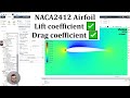
- Run simulations for zero and various angles of attack (e.g., 8 degrees), observing convergence of lift and drag coefficients.
- Compare CFD results with experimental data, achieving around 13% error in lift coefficient and 30% in drag coefficient.
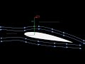
- Visualize velocity contours, pressure contours, and velocity vectors to understand flow behavior, showing stagnation points, boundary layer development, and lift generation through pressure differentials.
- Analyze y-plus distribution along the airfoil surface to confirm boundary layer capture.
Practical Insights
- Discuss mesh independence and domain size studies as pathways for result improvement.
- Highlight trade-offs between computational cost and simulation accuracy.
- Emphasize CFD’s value in predicting trends and enabling modifications without physical experiments. For a broader aerospace context, consider Understanding Aircraft Performance: A Comprehensive Overview of Flight Mechanics.
Conclusion
This tutorial equips users with a thorough understanding of airfoil simulation in Fluent, including geometry preparation, meshing, solver settings, and interpreting results under varying aerodynamic conditions. Feedback and requests for additional simulations are encouraged to enhance learning.
By following these steps, users will gain practical CFD skills to simulate airfoils accurately, analyze aerodynamic performance, and visualize critical flow phenomena. For a detailed step-by-step process, explore the full Comprehensive NACA 2412 Airfoil CFD Tutorial with ANSYS Fluent.
hey everyone and welcome to this tutorial for a NACA 2412 airfoil in ansys fluent we're going to go through
the full steps of creating the geometry the mesh on setting up the simulation in ansys fluent I'm going to do this
simulation in answer student so that anyone watching this video can conduct the simulation at home by simply
downloading answer student and conducting the simulation or by doing it on the full version also
in this tutorial we're going to calculate the drag coefficient the lift coefficient on the airfoil we're going
to also plot the velocity Contours the pressure Contours and the velocity vectors of the flow field
we'll also then change the angle of attack and show how that affects how we model the simulation in answers fluent
and we'll also show how varying the angle of attack will change the flow fields surrounding the airfoil so go
ahead and load up answers on your computer and let's get started with this tutorial so the first thing we want to
do here is drag an unsus fluid analysis system into the project schematic like so
now the first step is geometry so we need to go ahead and get the knockout 20012 airfoil curve and import that into
design modeler so how we do that is simply to look up on Google um airfoil
plotter naca2412 so here's our airflow
um we'll leave all these digits the same this basically is identifying that this is the naca2412 curve shape that we want
and a number of points here we're going to change this to 200 because we get the choice between 200 uh and 20 points so
we're obviously going to pick 200 as it's going to be just a little bit more accurate and also we're going to close
the trailing edge here because we don't want to Hull at the trailing edge here and in our curve as we're going to get
errors in our simulation then I'm going to go ahead and click plot here
and send to airflow plotter and one last change I'm going to make here is to change the chord to be 1000 millimeters
which is one meter as this is the standard size for airfoils and it'll make calculating the Reynolds number and
velocity just a little bit easier and so once that's done I'm going to click plot again
and my earphones ready to go and I'm going to click csv's file of coordinates so this will give us an Excel file that
will edit a small bit before we can import into design modeler so I'll download that file and then open it
okay now once I downloaded this file there's a few edits we need to make um to the file so we can actually import
this into design model so the first thing I want to do is get rid of all this stuff at the top here as there's no
need for it so I'm going to click this top row hold hold Ctrl and come all the way down sorry hold shift
all the way down to this row and I just want to delete all them rows there I'm going to insert two rows here one and
two on the left I'm going to change this left very left column here to be hashtag group
I'll explain this shortly and this next one would be hashtag points #x hashtag y
and hashtag Z so hashtag group this is essentially um the I believe it's the type of Point
um all I know is that we're gonna put in here the 0.1 for all of the coordinates here and that seems to work when we
implement it into ansys um so that's what we put in here for group number and then for Point number
uh we're gonna put in one two three four and all the way down until 200. so how I do that how I speed up this process here
is to do equals click the row above and then click plus one and then I'm going to drag this formula here so this little
green square here I'm going to drag that down all the way down to my 200 and first point
all the way down to here I'll remove this in a minute we don't need that camera line
and lastly then the Z coordinate and even though we are doing a 2d simulation uh we will just put in here Z
equals zero and as answers expects it in the file that we're going to upload so put in zero here drag that down all the
way to the end now we don't need any of this stuff here the camera line I think there's some
more stuff at the bottom comb line and chord line we don't need that delete that and one last change you
want to do here so you can see at the end here basically the point start to repeat itself and it goes back to 100
which is the same as the top coordinate because it's trying to basically indicate that it wants to close the
trailing Edge and but how we actually do that in ansys um design model is we remove this point
here like so I change this to one zero and then it will close the trailing edge of
the airfoil so we have a fully closed curve and that's everything we need to do here and to upload this file into
design modeler so I'm going to save this in my downloads as a very bad practice but nonetheless just for video purposes
so I'm going to call it naca2412 and I'm just going to call it a video because I have this file done before
uh this needs to be a text file in tab delimited format just like so
and hit save yes that's okay and our file is now ready to go to be
imported into design model all right now that we've created the airflow curve in Excel to import into
design model we're ready to go ahead and create the full geometry so to do that I'm going to right click on Geometry
hit properties I'm just going to change the analysis type to 2D as we're just going to do the
2D airfoil today then right click geometry and load up design modeler
once design model is opened up I'm going to look directly at the x-load plane and go to concept 3D curve and here
we're going to import the curve we just created in Excel so I first need to change my coordinates to millimeters
that's what we had our coordinate file in I'm going to go to downloads and I'm
going to click the file that we created I'm going to import that and hit generate and now the R4 file is
created here so I'm just going to click on Zoom to fit just to take a proper look at it and all looks okay here
um so now what we want to do is we want to create a surface from this curve and then later on what we'll do is we'll
remove the airfoil surface from our fluid domain so to do that what I need to do is go to
concept go to services from edges click the curve I hit apply and hit generate and
what you'll see now is we now have a surface representing our airfoil okay so now I'm ready to go ahead and start
making the fluid domain around the airfoil and for this case I'm going to do a c-shape domain you can do an O
shape domain too where you just make the domain of fluid a circle around it but I'm going to make a c-shape domain as it
converges a little bit better so a c-check domain is going to have a c in front of the Leading Edge and then a
square behind the Leading Edge so to create that domain I'm going to go to sketching create
I'm going to create a semi-circle then in front of the Leading Edge so Arc by Center
I'm going to click here at the origin but I want to click When I See This P here as that's letting me know that I'm
directly locked on to the origin whereas the C just lets me know that I'm coincident to the x-axis so once I see
the P I click and now I want to create the Arc of the circle to be in line with the y-axis so I click once I see this C
here and the same again down here click once I see the C to let me know that I'm fully in line with my Axis
okay let's add some Dimensions here so I'm gonna make this domain about 15 quarts and
surrounding the airfoil as I found from previous studies that this is sufficient and give accurate results so I'd like it
to be 15 chords from here till here from one end of the semicircle to the other so that means the radius of this circle
would be seven and a half chords which would be seven and a half meters because you remember we made the airflow to be
one meter in chord length so I'm going to make this seven and a half meters as the radius of the circle
now I'm going to create the rest of the domain which is just a square part behind it so I'm going to click here we
want to see the P to be locked onto that point create a horizontal line indicated by that h
uh Dimension this line to be 15 meters which is 15 chords rearward of the Leading Edge
now I'm just going to fully close the domain and it's important here that I click
once I see this C here just so I don't have to add in an extra Dimension and that's my domain fully closed
now there are a few more sketches that I'm going to add in here and to The Domain and that will help me with my
meshing later on so there are two extra lines that I'm going to add in here and and this will you'll see later on I can
add sizings to the to these lines later on and in the matching software and it makes the meshing far more structured
and far easier to Define so I'd like a vertical line here um at the at the sorry at the trailing
edge of the airflow not the Leading Edge so I'm going to create a line just like this and it's not exactly at the
trailing Edge right now so I'm going to Dimension this to be one meter from I'm just going to delete that that's a
vertical Dimension I'm going to create this to be one meter from the origin just like this and once that line is
created I'm going to extend it to the end of the domains by clicking modify it extend
and just that'll extend it to the end of the fluid domain and now I want a vertical line near the
Leading Edge of the airfoil but not exactly so I've found that if I create a vertical line that's about 80
millimeters in the case for this airflow for the naca2412foil and this is the case that I found if you're using a
different airflow it may be different and but for this particular case I've found to create a vertical line at about
80 millimeters from the origin here and gives pretty good results and in terms of a nice mesh so this line here I'm
gonna do 0.08 meters which is 80 millimeters and from the the origin here and then
I'm just going to do the same extend this to the end of the domain okay and they're the lines that I need
now um to properly Define my mesh in a nice structured way so once I've created my
sketch here I'm going to turn this into actual lines so to do that I'm going to go to Concepts lines from sketches and
just select the sketch we just created hit apply and then click generate and you'll see we have actual lines now that
we can do some more um interesting things with and once we have lines we can turn this
into a surface so to do that now I can go to concept and go to services from edges and select
all the outer edges of my domain so be careful of this very small line here and while holding control I select all the
outer edges of the domain and then hit apply and you'll see we get a Surface here
that we're going to use to represent our fluid surface but if you notice if you look in the
tree that answers has created a solid surface and we want a fluid surface this is going to represent our full fluid
domain so I'm going to switch this here to fluid and then hit generate okay now that I have a fluid surface what I
want to do is I want to remove the airfoil surface we created at the beginning from the fluid domain so we
have an airfoil shaped hole in our fluid domain which will represent the solid airfoil so to do that I go to create
Boolean I'm going to do Boolean subtract the target body is the fluid surface
and the tool body is going to be the airfoil surface now to select the air full surface what we need to do is click
the airflow here but you'll see answers actually selects the fluid surface we just created we don't want that we want
to select the airflow in behind that so we need to click this plane here and you'll see it highlights the airfoil
surface then I hit apply and then click generate and you'll see we're now left with a
fluid surface here with an airfoil shaped hole in the domain and this hole is representing our solid airfoil of
course now there's one more thing I need to do before I can bring this to the meshing
software and what I need to do is I need to split the domain into different faces and from the sketches that we created to
help refine our mesh so to do that I'm going to go to tools face split
select this face here and we're going to split the face by the sketches that we created so select the
lines that we created earlier on these lines here and we're also going to select the x-axis here so that we have
six total faces hit generate these six total faces now in our domain
that we can mesh separately now there also is one more thing I need to do and I was getting errors with this
small edge here so I'm just going to combine it with this larger edge here and as it makes it far more easier to
mesh so to repair this Edge what I'm going to do is I'm going to use the edge selection filter hold Ctrl click this
edge here and this edge here go to tools merge
and you'll see we have merge type as edges and then hit apply and click generate and what you'll see is now
instead of having that small line and the the larger line here this is all just the one line now all the way up to
this point here I'm going to do the same thing for this lower half of the domain
I'm going to click on this edge here hold down control and then click this edge here
tools merge and apply and click generate and just to check that that's merged the two lines together when I click this
line here this is my full Edge now which is exactly what I wanted so I'm ready to go here to bring this to answer smashing
so now it's time to properly save the file so properly saving files and answers is
really important if I go to file save as and save my project somewhere I really don't want to just save this to my
desktop or my downloads folder or even into my documents folder because what's going to happen is ansys is going to
save some extra files and alongside this file and if we just save it into a folder all these files
might get lost the files that we need to actually open our project so what we need to do is to create a working
directory or in other words just create a folder specifically for this project so what I'm going to go is what I'm
going to do is I'm going to go to documents create a a new folder here I'm going to
call this Nokia 2412 video and then inside that folder I'm going to
create a the project file and I'm just going to call that the same thing naka2412
video now if I go to my documents and look at the folder I created here you'll see
that where I save my project file which is the file we're working off here there's these extra files in here so
this is what I meant when I said that answers is going to save some extra files and we need these extra files in
order to open our project so this is why it's important to create a proper working directory and a designated
folder for your project otherwise these files are just going to get either lost or it'll be dumped into a folder where
you don't want them for example on your desktop in your downloads and in your documents folder so we don't want that
so it's really important you create this folder for your project okay so once that's done we have our project saved
and we're ready to move on to the meshing step start meshing I'm just going to click
edit and this load up answers mechanical once ansys mechanical is loaded up here I'm just going to look at the XY plane
again and as you can see here we have a line body from the sketches we created I'm
just going to go ahead and suppress that body as we don't need it anymore as we've split our domain into different
faces so there's no need for that now I'm going to add some edge sizings here to the mesh and to do this I used a
there's another tutorial on YouTube from a guy named Anthony T and I'm going to use the sizings that he used in his
video as he managed to get a very structured mesh with these particular Edge sizings and I'd recommend after
this tutorial if you're still struggling to model an airflow to go and look at his tutorial because it's very good and
so yeah we're going to use them Edge sizings in this mesh and then we'll determine afterwards if the mesh is
suitable to this airfoil so I'm going to insert a sizing here select these edges here while holding
down the Ctrl key hit apply change this to number of divisions
250 divisions and then I'm going to add a bias here select the first option and create a
bias factor of 50 000 and that's going to basically bias give us more elements towards the airfoil than the outer edge
of the domain but you'll see here that some of the edges are actually flipped in the wrong direction where we have
bigger elements close to the airfoil and smaller at the edge of the domain so we're going to go ahead and reverse all
the edges that are in the wrong direction and to do that we click on reverse bias hold down control and click
all the edges that are in the wrong direction and then hit apply now we're going to add some more edge
sizings here I'm going to select all three edges here hit apply
the number of divisions set this as 150 set the behavior too hard
and then create a bias again with a bias factor of 300 now and I'm going to reverse these two edges here
also now you'll notice I set the behavior as hard here and what this basically does
is it inflicts on the software a very stringy condition that we want 150 divisions here no more and no less and
that's what we do when we have a very simple shape that we're trying to mesh such as this square but as as before we
used a soft meshing condition as we're meshing multiple different edges and basically when we use the hard condition
we get a very structured mesh so we're meshing very simple structures it's it's okay to use this hard condition and we
get a very structured mesh but when we're using the soft condition and we might get as well as structured mesh but
we're less likely to run into errors with the meshing so in any other cfd simulations that you might be doing if
you're meshing a very simple shape such as a square or a rectangle and we can often use the hard condition and get a
very structured mesh but if it's a structure that's not very simple and then often using the soft condition for
the um element size behavior is often a better
option as then otherwise you'd run into errors using the hard condition nonetheless let's continue on with our
edge sizings here so I'm going to select these four edges here top and bottom of the airfoil and bottom
of the domain hit apply number of Divisions 150 here and set the behavior as hard
and then lastly we're going to select these four edges here at the outer edge front of the airfoil on the bottom of
the domain hold Ctrl and hit apply and we're going to do 100 divisions here for these edges with behavior as hard also
last thing we need to do is to add a face sizing here to let us the software know we want a quadrahedral mesh instead
of triangular mesh and to select all the faces just press Ctrl a on your keyboard hold Ctrl and hit apply and then click
generate and we'll take a look at the mesh so once the mesh has loaded we can
expect inspect it a little bit just have a look at how it looks and to be honest it could be improved a
bit more if I were to do this again I would probably reduce the length um of this point here towards the
Leading Edge of the airfoil so less than the 80 millimeters that I used maybe to 40 as What's Happening Here is I'm
getting kind of a squished mesh here and the the volume is going to change a lot from each cell from this cell to the
next one which is not what we want and these elements are also pretty skewed which is fine because it's far away from
the mesh but yeah there could be some improvements made to this mesh for sure but for purposes purposes of this study
I'm going to leave it alone for now because um
I'm just going to go ahead and get a solution and show you how to run a simulation rather than focusing on
getting the mesh perfect because mesh generation itself really is an art so the one last thing that's really
important that we do need to check and besides for mesh quality is take a look at the Y plus value um at the air for a
while so what the Y plus is is it's a non-dimensional value that lets you know how much of your mesh is capturing the
viscous sub layer so in order to capture this non-linear behavior of the Velocity profile at the wall you need to have a y
plus of one and the reason for that as you can see is this is a y plus value of one here and then as you as we go along
here we get this non-linear behavior all the way so in order to capture this non-linear behavior of the Velocity at
the wall we need to ensure that our first cell height is at what's called a y plus of one and we can use a
calculator in order to figure out what our y plus value should be so in other words how big should the Cell at the
wall be in order to capture this non-linear behavior of the Velocity at the wall and this is going to be
important for this airfoil simulation where we're concerned about maybe the adverse pressure gradient of the wall
and looking at the separation length across the airfoil so it's important to have a y plus of less than one and where
wall effects are important but for other simulations and where wall effects are not important it might not be need to be
captured so nonetheless for this simulation we're going to aim for a y plus of less than one and it will
actually be an output of the simulation because it's a function of the Velocity profile and we don't know the velocity
until we solve the final simulation and but nonetheless we can use calculator to get an estimate of what our y plus is
before we start the simulation we can then go ahead and calculate our solution and then we can get the Y plus as an
output to see if we've kept a y plus of less than one in the majority of the mesh so to calculate the what value
um our cell height needs to be to get a y plus of less than one of course we need to pick a Reynolds number of the
flow and the Reynolds of where I'm picking for this case is compared to this
experimental data um from Abbott and I will leave this also linked in the description so you
can have a look at this experimental data and run some different simulations yourself but here's a Naka 2412 airfoil
with the lift coefficient versus angle of attack and the dry coefficient versus the lift coefficient and there's a list
of Reynolds number here so I just picked an arbitrary Reynolds number of the first one here of 3.1 by 10 to the six
and by using this Reynolds number in our simulation we can then compare later on our lift and dry coefficients and to
this experimental data but nonetheless now that I know my Reynolds number for the flow I can calculate what the
velocity the mainstream velocity of the flow is so by rearranging the formula for the Reynolds number and this is
wrong for a day of viscosity here and I actually use 1.802 e to the minus 5 because this is air at 288 Kelvin
and using these values I got a mainstream velocity of 45.6 meters per second now to calculate what value
um our first cell height needs to be to get a y plus of one I can input these values into a calculator
so I used 1.802 e minus 5 here for the viscosity our reference length is going to be our chord length which is
was one meter as you remember and we want a y plus of one I need to put in the mainstream velocity here
45.6 and it's going to should be much smaller than this so
this is our value in meters so I'm going to convert this to millimeters just so it's a little bit easier to see um in
ounces so meters to millimeters so we need to have 0.008 millimeters and as our first cell height thickness so
I'm gonna go to answers here and let's take a look at the airfoil we want to zoom into the wall and try and
get an estimate of the first layer height so zooming in right down to the band layer what I can
actually do is press this selection here to select a node and if I select this node here and this node here you can see
that the the distance from the wall of the first cell height is equal to 6.3 e to the minus three millimeters and the
Wall height that we need to have a y plus of one is equal to 0.008 which is 8.2 e to the zero e to the minus three
so this value here is less than what we need for a y plus of one so we know that we have a y plus of less than one in the
bench layer and we're going to capture all the boundary layer effects and in our simulation and but of course I
think it it really is important to state that the Y plus is an output of the simulation so actually the Y plus value
that we just we just got is an estimate and the Y plus value that we we need sorry the cell height that we need to
maintain a y plus of one will actually change over the wall so it is important that we check this after the simulation
and ensure that a y plus has remained mainly below one um all around the airfoil wall
one last thing we also need to do is we actually need to create our boundary conditions
um for fluent so what I'm going to do here is I'm going to zoom in on the airfoil
select the edges of the airfoil here press n on my keyboard or actually what I should do is right click
and press create name selection just in case you don't have that shortcut enabled
we're going to name this airfoil and that's going to be our wall condition and we're going to select these outer
edges here all outer edges create a name selection and we're just
going to create this as our Inlet and then finally the edge here is going to be our Outlet
and now we're almost ready to go what we're going to do is we're going to press update and what this is going to
do is it's going to send the mesh to fluent and what that does is it gives us a green tick here on our mesh letting us
know that everything is done it's fully saved it's gone to um fluent so
file close meshing and I'm going to save the project one more time just before we go to the fluent solver
now I'm going to click on setup right click and press edit and we're going to start fluent
I'm just going to enable double precision and I'm going to use four cores here because I know I have four
cores on my PC and that's the limit on the student version as the maximum number of cores I can use and if you
don't have more than four cores or four cores that's fine and it's just going to affect how fast you solve your
simulation so once fluent loads up here we're ready to get going with our simulation
so once everything is loaded up I'm gonna go to General
and we're going to leave pressure based on steady for this simulation let's go to models and I have the sstk Omega
um model selected for the airfoil and this is a great model for predicting airflow separation especially when you
have a y plus of less than one and this is generally recommended for airflow simulations so I'm going to continue
using this model and for this simulation so now I'm going to go to material properties here just double click
materials go to fluid and have a look at the properties that I have for air here so the density is okay but I believe I
had a different viscosity so I used 1.802 as my viscosity so I'll change that here
thank you and hit change create so now let's click on boundary
conditions have a look at the inlet we have a velocity Inlet here which is exactly what we want
and just for good practice I'm going to change the velocity to be in components and we want the x velocity here to be
what velocity we had calculated for our rounds number which was 45.6 so 45.6 for our x velocity and hit apply
let's have a look and make sure that the name selections we created are all okay so the airflow here so there's a wall
condition which is correct and the outlet is a pressure Outlet and the gauge pressure here is zero so
that basically means that the pressure at the outlet is zero pascals above atmospheric pressure and how I know that
is if I look at operating pressure I'm operating at atmospheric pressure and then the gauge pressure would be the
value of both our operating pressure which is zero here which is exactly what I want the outlet is essentially at
atmospheric pressure which is what I want I'm going to leave all the settings alone here
I'm going to go to reference values and I'm going to compute from the inlet and this is important because we're going to
be calculating drag and lift coefficients and we need the values to be the same as the values we use at the
inlet otherwise our drag and lift coefficients will not be calculated correctly
now I'm going to go to solution methods I'm going to leave all the default settings here as second order upwind and
using the coupled and pressure velocity scheme I'm going to go to residuals
and I'm going to reduce this down to one e to the minus 6 because we're running a very simple kind of simulation here so
I'm I'm perfectly fine with um instructing a more strict convergence
condition on the residuals here so then we're going to go to initialization
however initialization is fine and you can use standard if you want all this basically does is
um solving the final volume method is an iterative solution so we need to assign the cells an initial value or an initial
guess and so that the simulation can proceed to continue so it doesn't really matter which initialization scheme we
use it just affects the path to convergence so I'm just going to use hybrid here and
initialize the solution okay once it's initialized we have a few more things we need to set up here so
I'm going to basically set up the drag and lift coefficients and to be an output of the simulation so we can look
at how they're converging so to do that I go to right click on report definitions a new Force report and we'll
do drag we'll change this to drag coefficient
keep it as dry coefficient and we're looking for a drag coefficient on the airfoil force Vector leave that alone
we'll talk about that when we change the angle of attack and we want to print it to console and
repent print a report file to so that's all okay so that's our dry coefficient done and now we just need to create one
for the lift as well so we're going to new Force report lift
click on air foil lift coefficient and we want to put this console 2 and
then click ok double click on Rune calculation and
let's just do one thousand iterations and that should be plenty for the solution to converge so that's
everything we need to Define and we're ready to calculate the solution so once I click on calculate then I
should get a graphic window showing me the lift and the drag coefficients and how they're converging with the number
of iterations and I should also be able to see the residuals and how they're converging
and as I said this is a very simple simulation so there should not be too many problems and with convergence it
tends to be with unsteady simulations or simulations with heat transfer or something like that that we might have
issues with convergence and so I'm not expecting any errors and or any difficulty in convergence of this
simulation and you can see we have the lift and dry coefficients also being reported to the
console and we'll compare these final values to the experimental data from Abbott
so here's our dry coefficient our residuals and our lift coefficient and I will know that the solution is
converged is essentially when this the values just are not changing too much from one point to the next
um and you'll you'll notice that the residuals will keep decreasing all the
way down to the value that we've set them to usually and but the lift and the dry coefficient tend to converge a lot
sooner so for accurate lift and dry coefficients we might only need a couple hundred iterations before the value of
the lift and the drag don't change too much more so you can see that the lift and dry coefficients have not been
changing for a while and but the residuals are still going down so I'm going to leave it for a while
um you can see yep here's our dry coefficient here on the left sorry our lift coefficient left and our drag on
the right so I can go ahead and check this against the experimental data while this is rolling just to see if we're on
the right track so if I go to the experimental data here for a zero degree angle of attack which is what we have
and in our test case for and for a Reynolds number of 3.1 million if I go up along this line here
and have a look at the circular Dot zoom in so zero degree angle of attack it's
quite difficult to look at and go across it's somewhere in between 0.2 and 0.3 for sure probably about 0.25
for the section lift coefficient and what we have here is a lift coefficient of 0.218 so in terms of error and to
experimental data here you're looking at about 0.218 divided by 0.25 which is about 13 error which to be
honest is quite good especially considering the fact that we haven't done a mesh independent study we haven't
done a a domain study so we haven't vary the size of the domain to have a look at how that affects the results and
nonetheless this is cfd this is a steady simulation there's lots of assumptions embedded in here and to compare that to
experimental data and get only a 30 13 error and I think it's very very good and especially for cfd
now let's take a look at the dry coefficient so we have something like 0.009 and if I look at the
data on the right here for a lift coefficient of 0.2 would be about here and I scroll up
the circular dot here for the drag is out about if I go across here is that about the line below is
0.5.6.65 0.0065 for the dry coefficient and you can see there's a little bit more error
here on the dry coefficient so if I go to calculator and do 0.0065 divided by 0.009
let's round that up to seven yeah about a 30 error so that's more like what we will kind of expect from
cfd results and I'm I'm pretty okay with Dem results especially considering we have not
looked into the wall effects too much we haven't put in a friction coefficient or anything so
um I'm quite happy with having a a dry coefficient of about 30 error here and especially given that the lift
coefficient is quite good so these are you you probably could get more accurate values than the values
I've got in here but again that would take uh doing a mesh Independence study doing a domain size study maybe looking
at some some more of the wall effects and improving the mesh quality and taking a look at time dependent effects
and there's lots and lots of different things we could do here to improve our accuracy but with improving accuracy
takes improved effort improved computational costs and so there is trade-offs to trying to get your your
answers as close as you can to experimental data and not only that experimental data and publish such as
this is not the end-all be-all some experiments are different than others or
is tolerances involved in error so we we can't take the values here as set in stone also so you can see that getting
values as close as we can and within the range with reasonable values and getting simulations that follow the same Trend
as the experiments is more than what we're aiming for rather than getting exact numbers from our cfd if that makes
sense so the main value in cfd is we'd expect that as we increase the angle of attack we should get a line similar to
this with a similar slope we should get similar values for our lift and drag and our simulations should follow similar
Trends to our experiments and then we know that we're simulating um our simulations are accurate in the
sense that the representative of the experiments and then the beauty of cfd is then once we know
that our simulations are accurately represent in reality for this case we should expect to change flow conditions
and then still be getting accurate results so I should be able to change the velocity to 44 or 43 down to 40 and
for the most part I should be confident in my results that um I'm representing reality properly so I'm put doing an
experiment for example and it might not always be available to change quantities dot easily or change the geometry that
easily so this is why we use cfd and this is why it's valuable so once the simulation is done let's
take a look at our results so moving down here to the graphics we can create a velocity contour and just
take a look at how the velocity field is behaving so I go to Velocity Contour I'm just going to give this a name
changes to Velocity and velocity magnitude is fine for now and just hit save display and it should
display the velocity um on this symmetry plane here so you can see what we get is we get our
velocity slowing down and reaching a stagnation point at the front of the airfoil and then we can we can see the
effect of the boundary layer being represented and we have our no slip condition after a while so this looks
quite good and then we get a little bit of Separation here at the the not really separation more just the flow and having
a discontinuity let's say at the trailing edge of the airfoil and then that affects the flow all the way back
to the edge of the domain for the most part so this looks quite good and now let's
look at the pressure and this is quite interesting because it I'll be able to explain how an airflow works so let's go
to pressure Contour static pressure is fine and display
so how an airflow actually generates lifts and how airplanes actually fly is what we get is you'll see we have at the
lower end of the airfoil and we have a region of higher pressure and above the airflow we have a region of lower
pressure so what we actually get here when we have low pressure is we have the airfoil airfoils top surface being
pushed upwards uh as it's being sucked by the low pressure whereas below here as you can see the green Contour
represents a positive pressure we should expect to see the force pushing the airflow up below so the way an airflow
works is we get a kind of a soaking Force upwards and a pushing force below and that causes a lift Force now there
is regions of negative pressure here and that's because we have a zero degree angle of attack and what you'll notice
is as we increase uh we'll move now to a different angle of attack and you'll notice you'll get a much more
pronounced effect between the a lower pressure region on top of the airfoil and a high pressure region below that
creates a much bigger lift force on the airfoil um so yeah essentially that's how
airflow works and we'll explore that by changing the angle of attack shortly but one more thing I want to look at before
I move on is have a look at the velocity vectors just going to call this velocity
vector and do it by magnitude again
and further velocity magnitude in this case I had to change the scale here to 10
before I could see anything and click fluid Surface body so the velocity magnitude is scaled by its actual
magnitude so we we have to play around with the vectors A little bit to get the size we want
so to more accurately visualize this flow I will change the vectors A little bit more
let's go in here to Vector options and do fixed length and hit apply and Co dot changes it
Okay so now the vectors are too big so I'll change this scale again back down to one
hit save display still too big so let's try 0.1 yeah it's starting to get a little bit
smaller now so let's maybe change this to 0.05 so depending on what angle of attack and
what airflow you're running sometimes the velocity vectors takes a little bit of playing around with before
um they make any sort of sense and in terms of how they look so I'll actually change
this right the way down to 0.01 and now this is much more clear so you can see the flow
comes in and we get sort of a stagnation region not really recirculation here but just stagnation then the flow will go
over the airflow we get zero flow at the wall of course due to the no slip condition
and then the flow here just continues on so I'm happy enough with these results and now we'll move on to a different
angle of attack so when we change the angle of attack in this simulation what we need to do is
we're going to um enforce components on the flow so for
example um given the angle of attack we're going to change the velocity component such as
the x coordinate to be um the velocity times the COS cosine of the angle and that we're going to be
simulating and then for the Y velocity of the component which was originally zero when we had a zero degree angle of
attack we'll change that to be the velocity magnitude times the sine of the angle and that were that we're
simulating and also what we need to do is we need to change the lift and drag Force vectors because the lift in the
drag is always measured perpendicular and parallel to the relative flow Direction so you'll see the lift is
always 90 degrees to the flow Direction and the drag is always parallel to the flow Direction so whereas before when we
were um we were defining the lift and dry coefficients we left the velocity I we
left the force components the same we're going to actually need to change them now in this simulation when we change
the angle of the flow so if we want to simulate say an 8 degree angle of attack on this airflow what we do is we go to
the velocity section and where we had an x velocity of 45.6 our x velocity is now going to be 45.6 times the cosine of 8
degrees so if I go to on my calculator 45.6 times cost of 8 degrees I get 45.156 as the component of velocity and
the Y velocity upwards is going to be 45.6 times the sine of 8 degrees and that gives me
6.346 and if you were to do calculate the magnitude of the x velocity squared plus the Y velocity squared and this
should still equal to the 45.6 that we originally had for a velocity magnitude so hitting apply now the flow will be
tilted in an eighth grade direction towards the airflow and we also need to change the force
vectors of the drag and lift coefficient to be parallel with the flow so or perpendicular in the case of lift
so if I go to report definitions and go to my dry coefficient as this is the most simple one to do we want the
drag Force Vector to be parallel with the flow and we know we've tilted the flow now 8 degrees so the force Vector
that's parallel with the flow is going to be cosine of 8 degrees in the X Direction and sine of 8 degrees in the y
direction so cosine of 8 degrees I'm just going to type it into my calculator is 0.99
and the sine of 8 degrees is 0.139 and hit OK and what I'm
essentially doing here is just changing the force vectors rather than being one zero along this direction now that
we're tilting the flow we need to tilt the drag Force Vector with the flow and just by simple trigonometry you could
work this out yourself using some simple trigonometry you can work out that this drag Force Vector here and has
components cost 30 sine 30 and the lift is going to be in the X component of the flow it's going to be minus sine of the
angle and in the Y component it's going to be the cosine of the angle okay so minus sine of 8 degrees here in the X
direction for that Force Vector is going to be 0.139 and in the y direction we're going to
have a cosine of 8 degrees and it's going to be 0.99 for the force Vector for the lift
coefficient now if I reinitialize my solution hit okay
we should get a flow at 8 degrees here and our lifts and dry coefficients and should represent the lift and drag for
an 8 degree angle of attack if we have a look at the simulation data here or sorry the experimental data at
an 8 degree angle of attack we'd expect the airfoil to have let's scroll along here so I'm getting about
1.05 by looking at the experimental data here if this line here is 1.1 for Lift coefficient somewhere in between here
will be 1.05 is what we'd be expecting for our lift coefficient
on for our dry coefficient if we go along here and go to a section lift coefficient of 1.05 would be somewhere
about here move our Mouse up go to this circle here this is
representative random number of three million 3.1 million go across here we can calculate our expected drag expected
drag is somewhere about 0.11 0.115 ish somewhere in between point
0.011 and 0.012 is what we're expecting for our dry coefficient so these are expected answers from the simulation
so clicking Rune here we should be able to get our answers and compare.2d experimental data
so having a look at the results here even after about 80 iterations we can see our lift coefficient is almost
exactly what we predicted there of 1.05 which is really good and to be honest that's probably just by chance
um and looking at the dry coefficient we got about 0.0014 so if there's anything I'm
noticing from my simulations here is that my dry coffee my lift coefficient is pretty good but my dry coefficient
um appears to be predicted a bit higher by the um by the simulation so that's one Trend I can notice here by running
different angles of attack so now my solution has converged and let's take a look at the results so I'm
going to take a look at the pressure Contour and you can see here we are getting the
results I described before we get a positive pressure below the airfoil that's causing the pushing force upwards
of the airfoil and we get a low pressure region above the airfoil this is a negative pressure that's causing the
pulling of the airflow which and this is what's creating the lift on specifically what creates a higher lift for a higher
angle of attack it's due to this flow phenomenon here now we'll take a look at the velocity
Contour save display and you see we get similar velocity
profile but the flow is starting to kind of tilt in this direction here and it's essentially as you increase the angle of
attack and once it gets to a certain point the airflow will stall which is where it reaches its maximum lift
coefficient and then any increase of angle of attack above that point causes recirculation of the flow of both the
airfoil and essentially the flow separates and you don't get any increase in lift and it becomes very unstable
now let's take a look at the velocity vectors and it won't even make the vector just a
small even smaller again so we can properly visualize this here so let's make this 0.05
and let's investigate the flow so as you can see we get the flow accelerating around the airfoil here
and our bench layer is being accurately represented by the no slip condition here and
I'm happy enough with the results here so what I will do also is I forgot to show how we check our y plus our final y
plus value for the simulation so I go to plots go to XY plot and create new I'm going to call this y Plus versus
location and if I go to turbulence and wall y Plus
and it's going to do it in the direction of the vector 1 0 which is what we want do it on the fluid Surface body and then
sorry we're going to do this on the airfoil not the fluid Surface body hit save plot and we have to see the Y Plus
at all locations so you can see I'm at the Leading Edge of the airflow we get a y plus of about one just after
1.041 which is just above one so it's it's fine to be honest and then it decreases along the airfoil and this is
where it's really important along the boundary layer here is what's being represented here and it goes down to
about 0.0 .007 so it's it's below one at all
locations uh here for the most part except for the spike here and so I'm very very happy and with the wall y plus
here so that was the uh NACA 2412 airflow simulated in ansys fluent and with the
full geometry tutorial full meshing tutorial and the full results tutorial and we had a look at the effect of
changing the angle of attack um on the airfoil so I hope you enjoyed and leave me a comment below if you'd
like any more simulations for me to do I'm more than happy to take your suggestions into account and do a few I
rather do 2D simulations to be honest because um this simulation here is anyone that
watches the video is able to conduct a simulation um but I'm happy again to do some more
3D simulations the same as before but nonetheless just leave a comment below of um any simulations you'd like to see
me do and I'd be more than happy to do them and thanks for watching
To create the NACA 2412 geometry, first obtain precise airfoil coordinates using an online plotter with around 200 points for accuracy. Adjust the chord length to 1 meter for standardization, then format these coordinates in Excel by adding necessary tags for ANSYS DesignModeler import. Finally, import the data into DesignModeler to generate a closed airfoil surface ready for simulation.
Set up a C-shaped fluid domain extending about 15 chord lengths around the airfoil to capture flow effects accurately. Include vertical lines near the leading edge (80 mm) and trailing edge (1 m) to aid mesh refinement. After sketching the domain, subtract the airfoil surface to create the flow space and split the domain into multiple faces to facilitate structured meshing and improved solution accuracy.
Apply edge sizing with biasing to generate finer mesh near the airfoil surface and coarser mesh farther away. Calculate the appropriate first cell height (around 0.008 mm for Re = 3.1 million) to properly resolve the viscous sublayer and achieve suitable y-plus values. Use a mix of hard and soft sizing in meshing to balance mesh quality and prevent errors while ensuring the boundary layer is accurately captured.
Choose the pressure-based steady solver with the SST k-omega turbulence model because it effectively handles flow separation near the airfoil. Input velocity components adjusted by the angle of attack using cosine and sine functions, set convergence criteria to residuals of 1e-6, and enable second-order upwind discretization for higher accuracy in solving flow equations.
Define the airfoil surface as a wall, the inlet as a velocity inlet, and the outlet as a pressure outlet at atmospheric pressure. Calculate the inlet velocity using the Reynolds number formula, resulting in approximately 45.6 m/s for Re = 3.1 million in this tutorial. Set air properties like density and viscosity appropriately to reflect realistic flow conditions.
Expect to see lift and drag coefficients converging after simulation, with lift typically within 13% error and drag within 30% error compared to experimental data. Visualize velocity and pressure contours, velocity vectors, and y-plus distribution to observe stagnation points, boundary layer development, and lift generation. Comparing CFD outcomes against experimental results helps validate the model's accuracy and identify areas for improvement.
Perform mesh independence studies and domain size investigations to balance solution accuracy and computational resources. Refine mesh near critical areas like the airfoil surface while keeping it coarser elsewhere. Understand that CFD effectively predicts aerodynamic trends and supports design changes without physical tests, but always consider trade-offs between simulation time and precision to optimize workflow.
Heads up!
This summary and transcript were automatically generated using AI with the Free YouTube Transcript Summary Tool by LunaNotes.
Generate a summary for freeRelated Summaries
Comprehensive NACA 2412 Airfoil CFD Tutorial with ANSYS Fluent
This detailed tutorial guides you through modeling, meshing, and simulating a NACA 2412 airfoil using ANSYS Fluent. Learn step-by-step how to create geometry, set mesh parameters, run simulations, and analyze lift and drag coefficients, including the impact of varying angle of attack. Practical tips on y-plus calculation and comparison with experimental data enhance your CFD skills.
Airfoil Basics: Understanding Shape, Terminology, and NACA Naming
This video covers the fundamental concepts of airfoils, including their definitions, key parts like leading and trailing edges, and how shape affects lift and drag. It also explains important terminology such as chord line and angle of attack, and breaks down the NACA airfoil naming system for better understanding of airfoil design.

Comprehensive Guide to NACA Four-Digit Airfoil Geometry and Coding
Explore the geometric fundamentals of NACA four-digit airfoils, focusing on mean camber lines, thickness distribution, and their mathematical representations. Learn how to calculate upper and lower surface coordinates and prepare for coding your own airfoil data program in MATLAB.
Understanding Aircraft Performance: A Comprehensive Overview of Flight Mechanics
This lecture delves into the intricacies of aircraft performance, focusing on flight mechanics, performance diagrams, and the calculations necessary for understanding horizontal flight. Key topics include minimum and maximum airspeed, range, endurance, and the impact of weight on performance.

Mechanical Properties of Fluids: A Comprehensive Guide to Bernoulli's Theorem and Applications
Explore mechanical properties of fluids, Bernoulli's theorem, and practical applications in this detailed guide.
Most Viewed Summaries

A Comprehensive Guide to Using Stable Diffusion Forge UI
Explore the Stable Diffusion Forge UI, customizable settings, models, and more to enhance your image generation experience.

Kolonyalismo at Imperyalismo: Ang Kasaysayan ng Pagsakop sa Pilipinas
Tuklasin ang kasaysayan ng kolonyalismo at imperyalismo sa Pilipinas sa pamamagitan ni Ferdinand Magellan.

Mastering Inpainting with Stable Diffusion: Fix Mistakes and Enhance Your Images
Learn to fix mistakes and enhance images with Stable Diffusion's inpainting features effectively.

Pamamaraan at Patakarang Kolonyal ng mga Espanyol sa Pilipinas
Tuklasin ang mga pamamaraan at patakaran ng mga Espanyol sa Pilipinas, at ang epekto nito sa mga Pilipino.

How to Install and Configure Forge: A New Stable Diffusion Web UI
Learn to install and configure the new Forge web UI for Stable Diffusion, with tips on models and settings.

If you found this summary useful, consider buying us a coffee. It would help us a lot!