Introduction
Curvilinear coordinates are an extension of traditional rectangular coordinate systems, allowing for a more flexible representation of points in space, especially in complex geometries. In this article, we will explore the concepts and applications of curvilinear coordinates, their properties, and their use in various fields including engineering and physics.
What Are Curvilinear Coordinates?
Curvilinear coordinates are a coordinate system where the coordinates of a point are defined by curves, as opposed to straight lines in Cartesian coordinates. This system is particularly useful when dealing with problems where the geometry of a system isn't easily represented by rectangular coordinates.
The Need for Curvilinear Coordinates
- Complex Geometries: Many physical systems and phenomena are best described in curvilinear coordinates due to their non-linear boundaries.
- Simplifying Calculations: Curvilinear coordinates can often simplify the equations governing a system, making them easier to solve.
- Application in Physics and Engineering: Many fields such as fluid dynamics and electromagnetism leverage curvilinear coordinates to model complex tasks effectively.
Types of Curvilinear Coordinates
Curvilinear coordinates can take various forms. The most common types include:
Polar Coordinates
Polar coordinates describe a point in a plane using a radius and an angle. Points are defined by two values:
- r (distance from origin)
- θ (angle from the positive x-axis)
Cylindrical Coordinates
In 3D space, cylindrical coordinates extend the idea of polar coordinates by including height as a third parameter:
- r (radial distance)
- θ (angular position)
- z (height)
Spherical Coordinates
Spherical coordinates are used to define points in 3D space based on two angles and a distance from the origin:
- ρ (distance from origin)
- θ (inclination angle)
- φ (azimuthal angle)
The Relationship with Traditional Coordinates
Curvilinear coordinates can be transformed into traditional Cartesian coordinates and vice versa. This is crucial for applications in physics where interaction between different coordinate systems is required. Let's explore some transformation equations:
- For polar coordinates:
x = r * cos(θ)andy = r * sin(θ). - In cylindrical coordinates:
x = r * cos(θ),y = r * sin(θ),z = z. - For spherical coordinates:
x = ρ * sin(θ) * cos(φ),y = ρ * sin(θ) * sin(φ),z = ρ * cos(θ).
Applications of Curvilinear Coordinates
Curvilinear coordinates find applications in various domains:
Engineering
- Structural Analysis: In civil engineering, analysis of curved surfaces necessitates the use of curvilinear coordinates for stress-strain calculations.
- Fluid Dynamics: Flow around objects is often better analyzed using curvilinear coordinates which align with the streamlines.
Physics
- Electromagnetic Fields: The behavior of electric and magnetic fields around non-linear objects is often modeled using curvilinear coordinates.
- Quantum Mechanics: The Schrödinger equation is sometimes easier to solve in non-Cartesian coordinates depending on the potential field.
Mathematics
- Calculus: Integration and differentiation in curvilinear systems often simplify complex problems in multivariable calculus.
- Differential Equations: Solving partial differential equations can be formulated more conveniently in spherical or cylindrical coordinates based on symmetry.
Transitioning Between Coordinate Systems
Transitioning between coordinate systems involves a change of variables and an understanding of the metric properties associated with curvilinear coordinates. The Jacobian determinant plays a crucial role in these transformations ensuring proper scaling during integration.
Gradient and Divergence
Understanding how to calculate gradient, divergence, and curl in curvilinear coordinates is essential. For example, the gradient in spherical coordinates will look different from the one in Cartesian coordinates:
- Gradient: The vector field's gradient can be computed by applying the chain rule and considering the Jacobian.
Area and Volume Elements
- Area Element: In polar coordinates, the area element is expressed as
dA = r dr dθ, which scales according to the radial distance. - Volume Element: In spherical coordinates, the volume element is expressed as
dV = ρ^2 sin(θ) dρ dθ dφ, which captures the spherical shell's geometry.
Conclusion
Curvilinear coordinates provide a robust framework for tackling complex problems across various fields. Understanding their definitions, applications, and relationship with traditional Cartesian coordinates is essential for engineers, physicists, and mathematicians. By leveraging these coordinates, one can simplify computations and gain deeper insights into the nature of different physical systems. In a world that often requires an understanding of non-linear relationships, curvilinear coordinates serve as a powerful tool in both theoretical and practical applications.
कि आज हमारा टॉपिक कर मीन इक्वल ट्रीटमेंट इसमें जो भूकंप फॉलो कर रहे हैं वह वेक्टर नॉलेज एंड इंट्रोडक्शन टू टेक एंड प्लेसिस
बाय नेम और यार स्पाइजेन श्याम शरीर की जो व तो कर्मी नियर कोऑर्डिनेटर क्या होते हैं सबसे पहले हम इसमें यह देखिए हम इसकी
आरपी लेंथ एरिया और इसके मुतालिक बाकी बातें भी करेंगे ग्रेड प्वाइंट करेंगे जैसे हम रेगुलर क्वार्डिनेट में यह सारी
चीजें इस करते हैं वैसे ही कर भी near point में भी डिस्कस करेंगे तो कर्म इंजीनियर कोऑर्डिनेटर को डिजाइन करने से
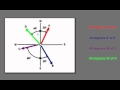
पहले हम एक छोटी सी एग्जांपल देखते हैं कि फॉर एग्जांपल अगर हमारे पास प्लेन में तो यह पॉइंट हो और एक्सांपल दिए पॉइंट है
इसके कंपोनेंट्स है यह भी है है और यह हमारे पास रेगुलर कंपोनेंट होते हैं एक्स एक्स और वाई एक्स इस तो यहां से
भी का मतलब यह है कि हम पहले एक्स एक्स स्क्वेयर लेंगे यह यूनिट लेंथ हमने कवर की फिर उपाध्यक्ष एसके लोंग बीच यूनिट लेंथ
कवर की तो हम इस पॉइंट पहुंच गए एडमिट लेकिन इसी पॉइंट तक पहुंचने का एक तरीका और भी था कि हम ऐसा करते कि हमने सर्कल
बनाते एक ऐसा सर्कल जिसका रेडियस यहां से यहां तक टोटल लेंथ होती हम उसे आरके देते हैं
हैं और साथ यह एंगल बी डिफ़ाल्ट कर देते हैं यह ऐंगल कितना अगर हम यह फील्ड स्टाफ और अर्थ भी डिफाइन करने मशीन और चेंज हो
जाने से यह पॉइंट आगे की तरफ जा सकता था और पीठा चेंज होने से ही पॉइंट किधर सर्कल के ऊपर किसी और पॉइंट पर भी जा सकता था
इसका मतलब इस पॉइंट को हमने एक नए क्वार्डिनेट सिस्टम की मदद से डिफ़ाल्ट कर लिया जो कि आर्थिक है यानी एक ही पॉइंट तक
पहुंचने के एक से ज्यादा तरीके भी हो सकते हैं तो इसी तरह अगर हम सफेद में बात करें एक्स एक्स एक्स वाई अक्षर एस और रिएक्शन
की बात की जाती है तो यह सक्सेस होगा अगर यह व्यक्ति भी हो और यह रिएक्टर्स को और यहां पर को यह पॉइंट के बीच सी हो तो इसे
भी सीटर जाने का मतलब यह है कि पहले हमने एक सक्सेसफुल लॉन्ग यह यूनिट लेंथ खबर की फिर हम वाई अक्षर के पैरलल चले और हमने भी
यूनिट लेंथ खबर कि यह है और फिर यहां से जेड एक्सेप्ट के पैदल चले और हमने सी यूनिट लैटर वकील हम इस
पॉइंट तक पहुंच गए तो जैसे वहां प्लेन में एक ऑडिट पैरों को लुक एट करने के एक से ज्यादा तरीके से वैसे ही स्पेस में भी एक
पॉइंट को लुक एट करने से एक से ज्यादा तरीके हो सकते हैं तो हमारा जो मेन मकसद इस चैप्टर में है वह यही है किस किसी भी
पॉइंट को एक से ज्यादा तरीकों से भी मुक्त किया जा सकता है तो जो नए क्वार्डिनेट बनेंगे उप जरूरी भी नहीं होता कि हमेशा
जोन क्वार्डिनेट कि उनके धर्म इन 3D पिंपल्स को कैसे का x-ray वायरस जो रिलैक्स दूसरे परपेंडिकुलर होते हैं हर 2
यह डाइट ढूंढ की मदद से डिजाइन किए जाते हैं कि एक्स एक्स और वाई अक्षर पर ₹90 के साथ और फिर रिएक्टर्स उसके ऊपर एक तीसरा
एक बनाया है जिसका उन दोनों के साथ एंगल नौकरी और है तो अब हम जो कर्वे नियर कोऑर्डिनेटर पढ़ रहे हैं उसमें यह जो
क्वार्डिनेट से इनका इस तरह से स्ट्रैट लाइन होना भी जरूरी नहीं है और इनका आपस में ऐंगल नौकरी डिग्री होना भी जरूरी नहीं
है लेकिन हमारे लिए अभी भी इंट्रस्टिंग वही होंगे है जो अड़हुल होंगे हम इसको डिफ़ाल्ट करें
और पार्टनर से क्या मिला दें ओके तो हम अब इसकी प्रॉपर्टी डेफिनेशन की तरफ आती है कि Let X वाइस चीफ आफ रैक्टेंगुलर
कोऑर्डिनेटर फॉर एनी पॉइंट्स पेट यानी स्पेस में कोई भी अपॉइंट है एक्स वाई सी एंड अट्रैक्टिव आइज विल बे एक्सप्रेस्ड
ठेर फंक्शंस आफ यू व्हेन यू टू एंड यू थ्री अब हम यह कोई नए व्यूअर्स इंट्रोड्यूस कटवा रहे हैं कि अगर हम
मेक्सिको ऐसा फंक्शन ओं q1 यू टू यू थ्री वालों को भी ऐसा फंक्शन आफ यू व्हेन यू टू यू थ्री और इसको भी ऐसा फंक्शन आफ यू
व्हेन यू टू यू थ्री डिफाइंड कर लें तो हम यह सपोर्ट कर लेते हैं यह जो हमने नए डिफाइन करवाया नए वैरियेबल्स इन कोर्स
करवाए हैं इन्हीं को फॉलो करते हुए हम यौवन को इन टर्म आफ थैंक्स वास जी लिख सके YouTube को भी इन टर्म आफ एक्टिवा इजी लिख
सके और यू थ्री को भी इंटर मोहन रॉय जी लिख सके तो यह कुछ इस तरह से निकलेंगे यौवन इज इक्वल टू यह क्रॉस इसका मतलब
सिर्फ इतना है कि युवा मिर्जापुर पैक्स वाले एंग्री सिमिलरली यू टू इज द फंक्शन ऑफ एप्स वाले ईंधन यूथ इज द फंक्शन
ऑफ वाइट एंड सी जैसे हमने भी एक्सांपल की है कि पोलर कोऑर्डिनेट्स की बात कर रहे हैं बेबी हैव यानी अगर मर तो यही पॉइंट्स
को मैं कह दूं एक्स वाय तो इसका मतलब यह एक सक्सेसफुल लॉन्ग हमने एक यूनिट खबर की ओर वाइफ इन उपायों में अगर मैं इस वक्त
ट्रायंगल को यहां दोबारा बना लो तो इसका मतलब यह है कि यह जो लेंथ है यह आ रहा है यह लंच हुआ है यह लंच अक्षय यह चल ठीक है
ओके तो हम यहां से इनको आपस में भी इंटर चेंज कर सकते हैं यह पॉइंट यह एक हुआ है और इस पॉइंट को हमने आर्थिकता तो यह जो
एक्स है और यह वाले हैं एक्स को हम इंटर मोगा रोड स्थित एक्सप्रेस कर सकते हैं देखिए कैसे यहां से एक होगा और को स्थिरता
और वायरल होगा और साईं थे टॉप ओ हाउ टो एक्सप्लेन द फंक्शन ऑफ और स्थिरता लिखा जाए तो हम इसे यूं लिखेंगे एक ऐसा
फंक्शन ओं करंट विटामिन और पॉकेट एंड व्हाई इज द फंक्शन ऑफ ऑल एंड थियेटर इज इक्वल टू आर साइन थीटा ओके तो ऐसी समझे
जैसे यौवन की जगह और YouTube की जरूरत है लेकिन अगर हम ठेर को इन टर्म आफ एक्स और वाई लिखना चाहे तो यहां लिख सकते हैं
देखिए कैसे के आर इज इक्वल टू 10 ग्लास हुआ है सोकर होल सोकर उठ उस एंपलीफायर करने से कोलर पार्टी नेतृत्व और फिर टाइप
होता है 10वर्ष वाइब एक्स यानी यहां यह जो आर है यह फंक्शन ऑफ एक्स एंड व्हाय है और यह जो है यह फंक्शन ऑफ एक्स और वाई है तो
यही बाद हम यहां किया कि हमारे पास लौंग 3 कंप्लीट से एक्स वाय और सीईए वह फंक्शन ऑक्युर व्हेन यू टू यू थ्री से और फिर
यौवन ऐसा फंक्शन क्वाइरी यह फंक्शन आफ फ्लाइज और यु टी इस फंक्शन आफ भाई सही है कि हमेशा भी पॉसिबल नहीं होता कि आप इनको
आपस में किन कर सकेंगे सिकलिंग यह दोनों एक दूसरे की इन्वर्स ट्रांसफॉर्मेशन से और इन ऐसा होने के लिए कुछ कंडिशंस का होना
भी जरूरी होता है जैसा के अभी हम कहते हैं कि आलथॉ थिस पोस्ट दैट इज द फंक्शन इन वन एंड टू और सिंगल वैल्यूड एंड हैव
कांटिन्यूज डेरिवेटिव्स अगर यह जो वन ओर टू है यह सिंगल वैल्यूड हो सिंगल वैल्यू सम्राट है कि हर एक पर्टिकुलर व्यक्त करने
से यौवन यू टू योर तरीके एक वैल्यू टूट करने से हमें एक्स की एक वैल्यू मिल वालों की भी एक वैल्यू मेरे और ही की भी एक
मीटिंग है इस पुस्तक को सिंगल वैल्यूड है और कंटिन्यूज डेरिवेटिव्स के यह डिफरेंस है
बंद हो इनके डेरिवेटिव पॉइंट किया जा सके और वह कंटिन्यूज पे हो तो फिर यह जो उनके धर्म इन कॉरस्पॉडेंस है वह वन होगी यानी
हर एक स्क्वायर जी के लिए हम एक यौवन यूथ फ्रंट कर सकेंगे और हर युग न्यू टू यू सिर ई केयर फॉर एडिंग एक्स वाई और रिफाइंड कर
सकेंगे ओके सो नॉट गिव विद रेगुलर क्वाइट सरप्राइज्ड टो सी यू नीड टो कोऑर्डिनेट यू आर यू थ्री अब इस पॉइंट को नए सिस्टम में
ऐड कर देंगे और यह जो क्वेश्चन नंबर वन और क्वेश्चन नंबर टू है यह तो यह ट्रांसफॉर्मेशन है जिसमें हम एक विघ्न हम
एक बॉडी सिस्टम से दूसरे कोडिंग सिस्टम में चले जाते हैं तो यह एक्सांपल है जब हम डिस्कस कि
कि एक्स वाय ए क्वॉर्इंट है इसमें यह लेंथ एक होगी बैलेंस उपाय होगी यह आ रहे यह ठीक है तो एक्सेस पॉइंट अंपायर और सीता सागर
मंथन किया जाए तो एक बार कॉस्ट तवा पुलाव साइन थीटा और डेल्टा को विंटर मोहित रॉय लिखा जा सकता यह स्पेस में यह मैंने से
प्लेन के लिए डिस्कस किया है स्पेस के लिए भी या के चलकर हमें एग्जांपल्स देखेंगे के स्पेस में किसी भी पॉइंट को यूनिफी एक नए
सिस्टम में को म्यूट कर पाया कि यूनीकली का वर्ड यहां मैटर करता है ओके तो है अब हम डिफाइन करते हैं क्वार्डिनेट
सर्विस इस ऐड कर दो कि आपके अगर यह वन ए कांस्टेंट हो YouTube यह कांस्टेंट फॉर ऑल यूथ क्लब यह
कांस्टेंट हो तो इनसे सरफेस बनेंगी है जैसा कि अगर हम बात करें प्लेन चपेट में चपेट में मार्ग पर सोते एक्स वाय और
री कंपोनेंट होते हैं अगर हम मेक्सिको एक और स्ट्रेट करें फॉर एग्जांपल एक्स इज इक्वल टू सीवन बल्कि अश्विन हमें और
स्टैंड मिक्स कर लेते हैं फॉर एग्जांपल यह है टू इसी तरह वायरल को अच्छी तो और भी घोल ऑफ और तो बेसिकली यह जो 30 इक्वेशन
लिखिए प्लेन जो है जो कि अ पर्ल है एक्टिवा प्लेन वायर्स प्लेन और सी एक्सप्लेन अगर हम इनको ड्रा करेंगे इक्वल
टू इक्वल 304 तो यह कुछ इस तरह से होंगे तो कि यह एक्स एक्स यह बाइक्स इस और यह जिससे
कि आपके एक्स इक्वल टू इट मींस नेक्स्ट ईयर लोंग टू यूनिट्स पर यह प्लेन है यह कुछ इस तरह है
लुटेरी ई-पेपर कि यह वाला है
मैं इसी तरह कि व इक्वल थ्री व्यक्ति पर भी यह प्लेन है 1243
है तो यह कुछ इस तरह से बन सकता है हु है और रिक्वेस्ट फॉर यदि आप लेने जो के
एक्स वाय है प्लेन के पैर ल ल ल में का ओके तो यह तीन बेसिकली प्लेन जो
हैं और यह जहां भी इंटर सेट करेंगे इनकी इंटरसेक्शन से लाइंस बनेगी यहां एक्सेप्ट नहीं किया जा सकता है लेकिन फिर भी आप
ट्राय करें तो यह प्लैन है यह कैसा प्लेन जो एक्स वाइफ प्लेन के पैनल है ऊपर की तरफ है यानी यह समझे कि यह आपका ग्राउंड है तो
यह आपके रूप है किसी कमरे की इसी तरह यह सवाल है जो के वायरस पर है और यह भी एक वाले जो एक्स एक्स पर है और जब भी कोई सी
दो यहां पर आपस में इंटरेस्ट करेंगे बल्कि अगर हम यह भी देखने के 101 बिलकुल जीरो यह वाला प्लेन है वॉइस प्लेन है वह बिलकुल
जीरो जो है वह आपके पास एक्सिस प्लेन है और जी कौन सी रोलेक्स वॉच प्लेन है और यह व्यक्तियों लंस आपस में इंटर सेट कर रहे
हैं तो उनकी मदद से स्ट्रैट लाइन बन रही है और यही हमारे रेगुलर क्वार्डिनेट से है है तो इसी बात को ध्यान में रखते हुए हम
कर मिलेनियर कोऑर्डिनेटर में यह बात करेंगे किसी 101 इक्वल सीवन YouTube तुलसी टू एंड ज्योति 793 आलोक डील आरएस
कॉर्डिनेटर्स और यह फैमिली इस अवसर पर सिद्ध होंगे मीन यहां पर सी1 और सी2 और C3 की वैल्यू चेंज कर देने से हमारे पास यार
डिफरेंट सफर सिर्फ बनेगी तो यहां इस तरह से इनको कोशिश की गई है कि ड्रा किया जा सके यह सिर्फ रसायनिक कौन सी वन यू टू
इक्वल सीटू एंड यूथ पीठ 793 ओके तो यहां यह जो यूं थ्री कुल सी टी और यु निकुल सीवन इन दोनों का जो इंटरसेक्शन है वह एक
लाइन होना जरूरी नहीं है बल्कि वह कोई कर भी हो सकती है जिसको अपने YouTube करो कहा इसी तरह यू टू इक्वल सीटू और दूसरी कुर्सी
थ्री इन दो सर्विस इसका जो इंटरसेक्शन होगा वह कर होगी जिसे हमने यौवन करो कहा यह कन्वेंशन के तौर पर हमने लिए हैं यह
चॉपिंग ऑफ थे इंटरसेक्शन 201 पहले यौवन और यु टी ई रिक्शा हंसी तरीका इंटरसेक्शन है उसे YouTube
पहले इसी तरह से यहां से यू थ्री करो ब्रिंग टू फ्रंट की गई है और आपके यहां सिर्फ इतना देखना है कि यह
सरफेस होंगी और इन सर्विस इसको हम कहते हैं क्वार्डिनेट तरफ से और इन क्वार्डिनेट सिर्फ इसके इंटरसेक्शन से जो कर उस बनती
हैं उनको हम यौवन कर YouTube पर और यु टी कर उसका नाम दे रहे हैं कि आपके यही बात यह की गई है कि द
कोऑर्डिनेटर प्रसिद्ध जनरली करूंगा एंड इट्स पर ऑफिसर फिर से intersect इन कर उस कॉर्ड कोऑर्डिनेटर करो और लायंस व लायनेस
स्वीकार्यता लेकिन यह स्ट्रैट लाइन होना जरूरी नहीं है 210 ह्यूमन कोऑर्डिनेट कर इस दैट लैंग्वेज
द ओनली वन वे यह तो एंड यूथस आफ कॉस्ट टो इसको यहां से तरफ देखा जा सकता है कि जैसे एक्सेसिव वहीं लाइन है यहां सिर्फ एक्स
वेरी कर रहे हैं तो आए और जी कांस्टेंट रहते हैं यह वैरी नहीं करते जैसे यह वाला जो पॉइंट है यह होगा1 शून्य से नेक्स्ट
पॉइंट 20 इसी तरह से आगे 400 को यहां एक्स सिर्फ वेरी करेगा हवाई और रिकॉर्ड होंगे इसी तरह वायरस पर एक सोर्स रीमिक्स रहेंगे
सिर्फ वाउ वेरी कर तय है और रिएक्शन क्यों इलेक्ट्रॉनिक्स रहते हैं सिर्फ यौन वैरी करता है तो इसी तरह यह बात की जा रही है
कि अगर हम अलार्म * कर देंगे तो सिर्फ यू वैरी करेगा का यूट्यूब और यू थ्री जो है वह कंस्ट्रेंट्स रहेंगे इसी तरह YouTube
चैनल और यु टी और यु वन कांस्टेंट होंगे यू तरीके लौंग यौवन और YouTube होस्ट होंगे
हुआ था ओके तो अब हम बात करते हैं कि यूनिट ट्रैक्टर्स क्या होते हैं तुम हमेशा इन कोशिश करूंगा कि इसको रिलेट करता रहा
हूं एक्स वाय और जी के साथ जब हम एक्स्ट्रा और एयरप्लेन में एक्टिवा 4g स्पेस में बात करते हैं तो एक्स एक्स के
अलार्म्स जो यूनिट वेक्टर होता है उसे हम आई सेड इनवेस्ट करते एक यूनिट वेक्टर होता है यानी एक यूनिट लेंथ ओरिजन से एक शख्स
की डाइरैक्शन में जो मेहर की जाए यह ₹1 तो वहां तक जो एक व्यक्ति है उसे हम आयु ने Twitter के थे इसी तरह वाई अक्षर के लोग
वन यूनिट तक जो व्यक्ति बनता है उसे हम यह यूनिट वेक्टर कहते हैं और इसके अलावा न्यूज नेटवर्क बनता है उसको हम कहते हैं
कि यूनिट फैक्टर और यह यूनिट ट्रैक्टर्स है यह म्युचुअली और पागल होते हैं आई डोंट यह
कि इक्वल होता है रीड ओह यह डौ 2004 के व्यक्ति इसी तरह आई डोंट आईटी कोल्ड नॉट यह
कि इक्वल के डाट की और यह वन होता है है तो इसी बात को ध्यान में रखते हुए क्योंकि अब हमने नए क्वार्डिनेट बना लिए
हैं तो उनके अकॉर्डिंग हमें न एटिन ईयर ट्रैक्टर भी चाहिए उन कंटेनर ट्रैक्टर की मदद से डिफरेंट करेंगे यह यूनिट वेक्टर्स
चाहिए इसकी मदद से उनकी डाइरैक्शन को सफाई कर सकें किसी भी पॉइंट की डाइरैक्शन को तो यही वादियां डिस्कस की जा रही है कि लेट
आर इक्वल एक ही प्लस वाई जेड प्लस जी के बीजों पोजीशन फैक्टर ऑफ़ पॉइंट्स पे यहां से पेश में कोई भी अपॉइंट है प्लीज
क्वार्डिनेट से एक्स वाय और सीईए तो क्योंकि हम रवींद्र कोऑर्डिनेटर में बात कर रहे हैं तो एक्स हम इन टर्म आफ यू
व्हेन यू टू यू थ्री वाले को भी और सीम्स टो बे इन टर्म आफ यू व्हेन यू टू यू थ्री एक्सप्रेस कर सकते हैं तो अब देखिए कि
एक्स जो है वह ऐसा फंक्शन ऑफ़ ह्यूमन यू टू यू थ्री है वायव्य फंक्शन आफ यू व्हेन यू टू यू थ्री फोर जीबी नगर फंक्शन आफ यू
व्हेन यू टू यू थ्री इट मींस आल ऑफ दिस इज एक्टिव वॉइस एंड सीआर फंक्शंस आफ यू व्हेन यू टू एंड यू थ्री एडमिन पहले जोक
की परमिशन ऑफ एक्स वाई और जी था खैर अब वहीं आर फंक्शन आफ यू व्हेन यू टू यू थ्री होगा ओके अट्रैक्ट 2018 इस पार्सल आरोग्य
व जो है यह ह्यूमन इसके ऊपर करेंगे यह इस दायरे में होगा तो यह होगा इसी तरह से तो इसका मतलब हमें में भी मिल सकता है उस
व्यक्ति का डिवाइड कर देने से divide करने से हमारे पास एक ट्रैक्टर है डायरेक्शन आफ पार्सल आर यू ओके तो अगर हम इस वाले
पोर्शन को 500 में लिख सकते हैं नेक्स्ट 9 न्यूज रूम चलो वन एंड होल्ड एडवांस या फिर इसे ओवन
को यहां मल्टिप्लाई करके लिख सकते हैं यह वन यूनिट वेक्टर इज इक्वल टू पार्ट्स आफ वर पर्फील ह्यूमन या फिर पास का अलार्म
वॉल्यूम अन इक्वल टू वन इवन हेल्थ यह यूनिट फैक्टर का यह इसी तरह जो यह जो YouTube पर है इस पर Jio 4G अट्रैक्ट होगा
वह का पार्सल आरोपी पार्षद YouTube और उस डाइरैक्शन में जो यूनिट ट्रैक्टर होगा उसको हम इनटू हिस डेथ नोट करेंगे और वह
व्यापार सैल और पार्सल यू टू डिवाइड पार्सल और पार्सल यू टू मेक नहीं चूरू इसको अगर हम X2 कहें तो हम लिखेंगे
पाठशाला Rover पार्सल यू टू इक्वल 828 सिमिलरली पाठशाला रुद्रपाठ व्यक्ति इज इक्वल टू थ्री लठ
कि आपके यह 18243 यहां पर हमने डिफाइन की हैं इनको निकाल सके न केवल फैक्टर्स हम एवं यहां यह तीन यूनिट वेक्टर्स डिफाइन कर
लिए 182 और रील तो इनके पेट्रोल और हां इनके पेट्रोल हम एक और सिस्टम भी इंट्रोड्यूस करवा सकते हैं ऑफ यूनिट्स
ट्रैक्टर्स है वन हेट यू टू हैड और 81 याद रहे कि यह जो जीवन है यह इंक्रीजिंग ऑफ ह्यूमन की डाइरैक्शन में के डिस्ट्रेक्शन
में यौवन इनक्रीज और है उसी डाइरैक्शन में इवन है यह डाइरैक्शन में यू टू इनक्रीज हो रहा है उसे डाइरैक्शन में * है और
डिस्ट्रेक्शन में यू थ्री इनक्रीज और है उसी डाइरैक्शन में भी 30 मिनट तक है हैं अपन
हैं अब बात करते हैं कि कैपिटल ह्यूमन कैपिटल यू टू और कैपिटल थ्री यहां तीन और वेक्टर भी किस तरह से डिजाइन किया जा सकते
हैं दिल्ली ईएमयू वन टू यह वह इस सरफेस के ऊपर जो ह्यूमन इक्वल स्टैंड सरफेस है उस पर एक नार्मल व्यक्ति होगा ऐडेड पॉइंट्स
पे है कि दोबारा देख लें कि जो इंग्रीडिएंट है किसी भी फंक्शन का ग्रेडियंट उस सरफेस
के ऊपर नार्मल होता है कि नॉर्मल इस पंचमी के वह उससे आउटसाइड नॉर्मल है इसी तरह यह जो जैल YouTube होगा
वह यू टू इक्वल सीटू सरफेस पर नार्मल होगा इसी तरह W3 यू थ्री खोल C3 सरफेस पर नार्मल होगा अगर वह नॉर्मल हैं तो उस
नार्मल की डाइरैक्शन में भी या नहीं यह कुछ इस तरह से है कि यह जो सरफेस है यह हमारे पास सिर्फ ऐसे यू थ्री सरफेस इसी
तरह यू थ्री कुल सीईए इसके ऊपर जो नार्मल व्यक्ति है उसे इस तरह से डिजाइन किया गया यह इसी के लिए जो टोटल आगे की तरफ जाता
हुआ फैक्टर यह W3 है लेकिन उसका गर्म यूनिट वक्त ले तो उसे हम MP3 कैपिटल a38 से डिफाइन करें इसी तरह बाकी दोनों सर्विस
के लिए भी कैपिटल * है ठेर कैपिटल वन हेट तीन नए यूनिट फैक्टर डिफाइन किए जा रहे हैं
यो यो हनी कैपिटल जीवन है दैट इज इक्वल टू दिल्ली ओवन डिवाइड मेग्नीट्यूड आफ डिन ह्यूमन इसी तरह कैपिटल * है ट्यूसडे
YouTube डिवाइडेड बाय न्यू टू मेक यू एंड थें हे गूगल W3 डिवाइडेड इनटू थ्री मेग्नीट्यूड
कि आपके खानी हर एक पॉइंट पर 10 सिटीज फॉर योर कन्वीनियंस सिस्टम दे रिक्वेस्ट इन जनरल टू सेट्स आफ यूनीक फैक्टर्स के हर
पॉइंट पर किसी भी पॉइंट्स को अगर हम देखें तो उस पॉइंट पर हमारे पास दो कि संघ ए यूनिट ट्रैक्टर्स मिल रहे हैं एक स्माल
इवन व्हाईल टू संभाली थी ईएस और दूसरा कैपिटल जीवन कैपिटल यू टू और कैपिटल भी तीन यह जो संभाली 1823 है यह यूनिट है
यूनिट वेक्टर से अ यूनिटेंडेड ट्विटर से इसी तरह यह कैपिटल ह्यूमन कैपिटल लेटर कैपिटल उतरी है यह भी यूनिट प्रैक्टिस यह
लेकिन यह नार्मल टू द क्वार्डिनेट सरफेस है ओके इनको इसी तरह से देखा जैसे आई जे और के होते हैं लेकिन वह सिक्स रहते हैं
किसी भी पॉइंट पर आई जे के वह SIM रहते हैं जब तक यह चीन इन की डाइरैक्शन है यह बदलती रहती है यह क्योंकि कर उसके ऊपर
होते हैं लेकिन इन के दरमियान जो अगर यह ऑर्थोंगोनल होंगे आपके हम यह टॉपिक्स डिस्कस करने लगे करिए और पागल होंगे तो
फिर यह सीआईडी और के की तरह एक्जेक्टली बिहेव करेंगे क्योंकि ID और के यूनिट सर्टिफिकेट
दरमियां सहगल नौकरी रहते हैं ओके तो अब हम डिस्कस करते हैं कि व्हाट इज और चैनल को कर्विलेनियर क्वालिटी में है
मैं इतना कोऑर्डिनेटर फीचर्स 1777 यू टू इक्वल सी टू यू 323 intersect अट राइट एंगल्स कि अगर यह वाली जो कर उस है यह जो
तीनों सॉरी यह सिर्फ इस है अगर यह राइट एंगल पर इंटरनेट करेंगे अब स्किन इंटरसेक्शन से सब्सक्राइब प्लेन बनेंगे
अगर वह आपस में राइट एंगल के साथ मिल रहे हो तो हम यह कहेंगे कि वह जो सर्विस है और वह भूल कर भी न कोऑर्डिनेटर है वह और
फाइनल हैं यह 91वीं के साथ है या हम इसको इसी तरह से बी डिफ़ाल्ट कर सकते हैं कि देकर मिलिए अपॉइंटमेंट यू आर यू टू यू
थ्री ऑल सेट टो अपीयर फॉर * ई एम इस द एक्टर्स इवन ई दो ई थ्री फॉर मैन और फिर नार्मल ट्राइड यह जो तीन वेक्टर्स है अगर
यह आई जेल के भीतर एग्जेक्टली बिहेव करें किसी भी पॉइंट पर यह कैसे कि अगर यह 12122 83830 और इनका क्लास प्रोडक्ट्स जो है
युक्ति दो ए गोल - * क्रॉस ईवन इक्वल टो MP3 हिट और इसी तरह एक बात और भी के 122 इक्वल हो गई थ्री लौट तो एक युद्ध 223 लें
और यह सारे गुर्जरों पर यह आप उसमें पर्टिकुलर हूं तो भी हम यह कहते हैं कि वह जो कर क्लियर कोऑर्डिनेटर है वह और फाइनल
है या हम इस तरह से 20 इसी बात को दूसरी तरह भी लिख सकते हैं कि फिल्टर टेस्टी 18238 पॉइंट्स पेटू यूथ को-आर्डिनेटर
लाइंस फ्रॉम दिस पॉइंट अ म्यूचुअल परपेंडिकुलर के यह आपस में रूचि परपेंडिकुलर होंगे इसलिए पर्टिकुलर का
मतलब है कि हर दो आपस में परपेंडिकुलर हैं कोई से दो वन ओर टू यू टू और थ्री लिए और जीवन भी तो हम यह कहेंगे कि यू यू थ्री जो
क्वार्डिनेट सिस्टम है वहीं क्विंटल कोऑर्डिनेट सिस्टम है कि आपके अब तो अगर हमारे पास और फाइनल
प्वाइंट सिस्टम हो तो हम किसी भी व्यक्ति को ऐसे और रेगुलर कोऑर्डिनेटर में किसी भी व्यक्ति को लिखते थे वेस्टर्न रेलवेज
इक्वल एवं नेक्स्ट एवं आई ए प्लस ए टू जेड ए प्लस थ्री के थ्रू यह उसका आयुक्त
कंपोनेंट गैस कंप्लेंट एंड डकैत कंपोनेंट या फिर इस तरह से भी लिखते थे एक साइड प्लस वाई ज़ेड प्लस जी के उसी तरह यहां भी
किसी भी व्यक्ति को इस तरह से लिखेंगे वहां यूनिट ट्रैक्टर्स आई जे और के थे तो उसके कंपलेक्स के साथ आई जे के यूज करते
थे लेकिन यहां हमारे पास यूनिट वेक्टर है वहीं 18233 है और सातवें से यह भी है यह तो इसलिए अगर वह परपेंडिकुलर होंगे तो
इनका भी आप उसमें अंग लाइन की डिग्रियों का यह भी म्यूचुअल ईईए अब पागल होंगे तो हम चैप्टर 1 को इस तरह से लिख सकते हैं
1111 हैड प्लस टू हैड क्लासेज या फिर ऐसे भी लिख सकते हैं एवं यह संभाले वन सिर्फ इनमें और इसमें डिफरेंस मेंटेन रखने के
लिए मेंशन किया कि यह दोनों मुख्तलिफ प्लस टू हिटलर से थ्री लैंड व्हेयर कैपिटल 183 हिमालयन
MP3 ऑल द रिस्पेक्टिव कंपोनेंट्स ऑफ वे इन विच सिस्टम यूज करेंगे तो उनके लिए डिफरेंट चाहिए
है लेकिन इसी लैटर को हम इनकी मदद से बे डिफाइंड कर सकते हैं कैसे के विक्टरी रिक्वेस्ट हमको स्टैंड पर चला Rover
पार्सल ह्यूमन प्लस हम कॉस्ट पर चला रूल YouTube प्लस कांस्टेंट फॉर सिल्वर 503 मी C1 अल्फा वन प्लस सीट वेलकम टू प्लस
सीरियल फत इन इसको अल्फा-1 कहा गया इस गोल्फर टू सपोर्ट कर लिया गया और इसको अख्तरी सपोर्ट किया गया
है यानी हम यह कह सकते हैं कि लैपटाप इज इक्वल टू पार्ट्स अलार्म व पार्सल यूपी यह भी एक जस्ट नऊ टेंशन के तौर पर लिया गया
कि यहां बजाय इसके कि हम यह तीनों अलग-अलग लिखे के अलावा ने इक्वल टू कैश विड्रॉल पर शिव वेलकम टू इज इक्वल टू दूसरे डाल पाती
इक्वल टूरिस्ट यहां रिजर्वेशन लिख दिया गया वापिस 2012 और तीन कि उसके तो यह जो है इनको हम कहते हैं सी1
और सी2 और यह C3 जो कैपिटल में लिए गए इनको का जातक कंट्रा वैरीअंट कंपोनेंट्स ऑफ यह टेंशन लेस में आगे आप देखेंगे कि
कंट्रोल वेरियंट और को बेगमपुर इसमें क्या डिफरेंस होता है इसी तरह हम वेक्टर एक को दिल्ली ओवन w2 और व्यतीत मदद से भी रिसेट
कर सकते हैं लिखेंगे सीवन बेटा वनप्लस 6 टू मी टू प्लस सीट 323 और यह जो कॉन्टिनेंट्स होंगे सी1 और सी2 C3 इनको
कहा जाएगा कंट्रोल वेरियंट कंपोनेंट्स ऑफिस मैं एक चीज और देखिए कि मैं यहां कहा कि
वे कैन अलसो रिप्रेजेंट व्यक्ति के इंटरनेट जॉब्स व्यक्ति हदीस विचक्राफ्ट यूनिटरी बेस वेक्टर्स इनको यूनिटी बेस्ट
प्रैक्टिस कहा जाता है लेकिन जरूरी नहीं होता कि यह यूनिट ट्रैक्टर हो तो बीच दक्षिणी सूडान होगी लेकिन हम पहले देख
चुके कैपिटल ईवन और अगर हिमांशु डॉन होगी तो फिर यह इस तरह से और देंगे अगर इनकी मिनिट बनोगे तो करिए कुछ इस तरह से हो
जाएंगे लेकिन यहां यह SIM को नाम के तौर पर यूनिटी फैक्टर कहा गया और नाइन का यूनिट वेक्टर्स होना जरूरी नहीं है
लुट ओके अब बात करते हैं कि और प्लैनेट्स को कैसे डिफाइन किया जा सकता है इसमें रैक्टेंगुलर यह जो कर भी नियर क्वार्डिनेट
से इसमें रेगुलर पर कैसे सेट करते हैं पहले तो यह देखेंगे कि हमारे पास अगर यह कर्व चेंज हो रही है यहां से यहां तक कि
तो यह उसकी और प्लांट होती है और हिसार के फैंस को हम इसकी जो टोटल डिस्टेंस है डीएसएन चेंजिंग डिस्टेंस से शेयर करते हैं
और यह कुल होता है डीआर डॉट त्यौहार में अपनी चोट का शुक्र इसी तरह से जब भी MS Word इन्हें इसमें हम ट्रेवल करेंगे एक
पॉइंट से दूसरे पोंछे तक तो उसके कुछ और प्लैनेट्स होगी तो उस आफ क्लांस को कर्विलेनियर कोऑर्डिनेटर में कैसे डिफाइन
करना है तुमको देखते हैं लुट ट्विटर और इज इक्वल टू फंक्शन आफ यू व्हेन यू टू एंड यू थ्री अगर हम यहां इसका
डिफरेंशियल लें तो उसको लिखेंगे दिया रिसीप्ट उपाय सलाद और फलों वन डे यू वन प्लस पर क्रॉस यूट्यूब यूट्यूब प्लस 5950
3D 3D यह पिन की मदद से डिजाइन किया गया यह calculus कि किसी भी मुल्क में आप देख सकते हैं मल्टीवेरिएबल कैलकुलेट से
रिलेटेड है ओके अब क्योंकि हम यह जानते हैं कि जो जीवन है वह बिल्कुल होता है पार्षद व
पार्सल यौवन डिवाइड मैनेजमेंट इसी तरह टू हेट स्टोरी 3 है डिफरेंट किए जाते हैं तो हम यह देख सकते हैं पार्सल व पार्सल यूआई
इज इक्वल टू एचआईवी-1 है हम पहले पढ़ चुके आई वांट टू या f-35 किया जा सकता है तो यही डीआर यह जो पार्सल आरओ व पार्सल
ह्यूमन है इसकी जगह मिलेंगे इन वन हैंड पार्सल व पर्स लूट को रिप्लेस करेंगे च्युई दहिसर पाठशाला Rover पार्सल यू थ्री
को रिप्लेस करेंगे ऐड 338 के साथ है तो अब यह जो डीआर है यह इस तरह से लिखा करो कि यह जो यूनिट वेक्टर है अगर हम किसी
भी एक यूट्यूब शैंपू चीज बनाना चाहिए तो उसकी एक लेंस यह है एच वन बी एच वन एन वन हेट इसी तरह दूसरी डायरेक्ट दूसरी
डाइरैक्शन में व्यक्तित्व यह टू डू यू टू हैड और तीसरा झुकती रिड्यूस 338 ओके और इसको कट कर रहे हैं हम आगे चलकर एक ऐसा
क्वेश्चन भी करेंगे इसमें हम इसको नार्मल कोऑर्डिनेटर में डिस्कस करेंगे अभी फाइनल कोऑर्डिनेटर के लिए देखते हैं कि यह पॉइंट
से है इसलिए 12283 और 310 होंगे तो यह टिप्पणी और इसी तरह अग्नि-1 अग्नि-2 अग्नि-3 है
ए डेट सूखे एयरक्लीनर के लिए फॉर्मूला होता है डीआर डॉट यार तू यही को लगा दिया कि हम लुट करेंगे और उसका अपने आपके साथ
डॉट प्रोडक्ट लेंगे तो दो प्रोडक्ट लेते हुए फर्स्ट कंपोनेंट को कस्टम पॉइंट से तो यह बन जाएगा एडवांस कार्डियक वंशों के
प्लस टू सोकर ड्यू टो स्केर प्लस 30 डीईसी 30 या हम डिस्कस लिख सकते हैं इक्वल सके रूट ऑफ़ 409 प्लस फिर ड्यू टो उसके प्लस
30 ड्यूएट्स ऑफ़ करो तो यह हमारे पास आर्ट क्लास के लिए एक्सप्रेशन है आगे चलकर जवान क्वैश्चंस को सॉल्व करेंगे तो उसमें यह
काफी मुश्किल होगा अ ओके तो इसके साथ ही एरिया एलिमेंट को भी डिस्कस किया जा सकता एरिया एलिमेंट कैसे
के यह हमारे पास घूमने क्यों बना रखा है इसकी किसी भी एक साइड का अगर हमने ये रिमाइंड करना हो तो वेक्टर में हमारे पास
फॉर्मूला होता है कि अगर हम यह तय मैं कर लूं ग्राम हो या यह सूखे एयर हो और ग्राम पुलिस का यह वेक्टर यह हो और यह
वेक्टर भी हो तो इसका जो एरिया होता है एरिया के लिए हम फॉर्मूला यूज करते हैं यह क्रॉस बीम एक नींबू तो इसी तरह से यहां से
जो एरिया एलिमेंट हमें मिलेगा और एग्जांपल हमें इसका एरिया चाहिए यह वाला एरिया चाहिए तो इसके लिए हमारे पास एक ट्रैक्टर
यह है और एक व्यक्ति और यह है इन दोनों का क्लास प्रोडक्ट्स लेंगे इसी तरह यहां यह जो नीचे वाला है इसके लिए इन दोनों का
क्रास प्रोडक्ट और इस साइड वाले के लिए इन दोनों का क्लास प्रोडक्ट्स लेंगे तो हम यहां डिफाइन करते हैं कि डे वन इज इक्वल
टू एरिया एलिमेंट विच साइड वेक्टर्स शेडच्यूल स्टूडियो टू हेज़ को यौवन कर भय उसकी बैक साइड वाली जो है यह जो यौवन
सरफेस है उस साइड पर जो एरिया एलिमेंट है वह यह है न यह यौवन कर्तव्य को इस कि बैक साइड पर जो पीछे
शुभेंदु सिर्फ इसे यहां पे जो है अगर मैं यह पिछले वाला पीस उठा लूं कर दो
कि यह देखिए कि जैसे हम यौवन करो कि बैक साइड में जो सफल है वह यौवन सर फिर से इसी तरह YouTube पर की वेबसाइट पर जोसेफ है वह
यू टू सिर्फ ऐसे और यू थ्री करो कि बैक साइड के जो अवसर पर है वहीं दूसरी तरफ है अगर हम उसके एरिया को डिस्कस करेंगे यौवन
की बैक साइड वाली सरफेस के तो उसके रिकॉर्ड 11:00 करेंगे इसी तरह YouTube की बैक साइड पर da2 और यु टी की वेबसाइट पर
डिटेल थी ओके है कि सोहम लिखने के लिए वन इज इक्वल टू एरिया एलिमेंट विच साइड व्यक्ति एप्स टू
यू टू हेल्ड इन 3D थर्ड तो हम फॉर्मूला पर चुके हैं कि एरिया का फॉर्मूला उत्तर लो जो साइड हैं उनके क्लास प्रोडक्ट्स कम
मेकेनिक जो तो इनके प्रॉडक्ट्स लेंगे सपोर्ट ड्यू टू हेट और 338 और फिर उसका मेकेनिक लेंगे अब इसको लिख सकते हैं अ
जूतों के पोस्टर बॉय लिखा जाएगा 13 भी ड्यू टू ऑडी Q3 भी तो वेक्टर है यह टू और थ्री सोम मेग्नीट्यूड आफ युटेरस की 3253
को है जीवन और जीवन का निचोड़ वन नाइट में इसका मेग्नीट्यूड भी वन होगा तो हम इसको लिखेंगे डे वन इज इक्वल टू मच दोएस 3D यह
एक बात यह पता चली कि जिस जॉन साधे लिमिट लेना है उसके दोनों साइड वाले जो शक्ल फैक्टर्स है
है और ड्यूल वन डे यू टू यार जो भी है जो सकते होंगे वहीं ड्यू आपस में मल्टीप्ल होंगे तो वह में एक एरिया एलिमेंट मिलेगा
इसी तरह धो और एलिमेंट की बनाए जा सकते हैं da2 जो के क्लास प्रोडक्ट्स का या 1431 अधिनियम-2011 हेल्ड एक्रॉस थे स्टेट
3-day जो 338 और यह लिखा जाएगा चेक्ड जीवन व्यतीत बाकी रहेगा ब्लैक निचोड़ में योग बन कर आती थी जो कि टू होता है और यह तू
मेकेनिक जुबान तो इसलिए एंड सिमिलरली ए टी उनको टेकऑफ है है तो यह हमने एरिया एलिमेंट डिफाइन के
किसी भी साइड का एरिया इस तरह से हम पॉइंट करेंगे ओके तो अब बात करते हैं वॉल्यूम एलिमेंट की एक किसी भी चीज का जो वॉल्यूम
होगा वह कैसे सेट किए थे कि देखिए अगर हमारे पशोपेश में वैसे रेगुलर कंपोनेंट में अगर ए क्यूब जो कोई भी एक पल उपलो से
कुछ इस तरह से बनाने की कोशिश करता हूं मैं हुआ है
हुआ है लुट कि यह अगर और इसकी जो तीन साइड से एक को
हम कह देते हैं जैसे स्वैप्ट अवे मैं एक मेज़ वेस्ट बी हैं और एक और जो है यह वाली साइड किसको
कहते हैं व्यक्ति तो इस जो अगले पर बनी है इसका जो वॉल्यूम है जो इसके इनसाइड है उसके वॉल्यूम का फॉर्मूला होता है यह डाट
बीच राशि और फिर इसका वृक्ष टूट मोड़ लिया जाता है जो कि एक सर्कुलर नंबर आता है तो उसका भी मोड़ लिया जाता है तो यह हमारे
पास वॉल्यूम मिलता है या इसमें से कोई भी एक व्यक्ति के यहां और बाकी दो इस तरह से यह लिखे जा सकते हैं जो कि हम और ले रहे
हैं इसलिए नेगेटिव पोस्टिंग को इफेक्ट नहीं करेंगे तो इसी तरह हमारे पास यहां जो शेप है उसमें हमारे पास एक साइड है अचीव
वन हैंड दूसरी साइड है एटीट्यूड यू टू है और दूसरी साइड इफैक्ट्स 3D थर्ड इस तरह एक का बाकी दोनों क्रास प्रोडक्ट के साथ डाट
प्रोडक्ट लेकर और उसका मेकेनिक छूट है यह मैंने फॉर्मूला पिछली साथ लिख दिया है तो यहां से ज्वाइन कांस्टेंट है टू
कॉस्ट है थ्री कॉस्ट यह चले जाएंगे डीयू वन इंडिया YouTube और व्यतीत यह मोड केंद्र रहेगा इवन हे डिड नॉट टू क्लासेज
अब इन टुकड़ों C3 होता है वन सो इवन नॉट गिव वन ई डी टीवी वॉल्यूम एलिमेंट हमारे पास इक्वल हुआ S1 S2 S3 लीड यू वन इंडिया
YouTube वीडियो 3G को योनि वॉल्यूम जो है वह इनका प्रोडक्ट है एच वनस्पतियों सर्कल फैक्टर्स और उनके
साथ डू यू वंट ड्यू टू डू तीन तो यह फार्मूले भी हमें कुछ मेमोराइज करना होंगे ताकि आसानी रहे ईद 1283 तीनों और आप तीनों
ही डू डू डू डू डू यू टू बी थर्ड जीवन में S2 S3 वह मीटिंग है वन वाला ओके इनटू ए धूल अमित सिंह और डी3 मिथलेश सिंह ने
अजय को
Heads up!
This summary and transcript were automatically generated using AI with the Free YouTube Transcript Summary Tool by LunaNotes.
Generate a summary for freeRelated summaries

Understanding Rectangular and Polar Coordinates for Advanced Function Analysis
Explore the complexities of rectangular and polar coordinates, their differences, and functional behavior in advanced mathematics.

Understanding Vectors: A Guide to Motion in Physics
Explore the significance of vectors in physics, their applications, and how to graph them effectively.
Understanding Vector Direction with North, South, East, and West
Learn how to describe vector directions using cardinal points effectively. Improve your understanding of geometry and vector analysis.
Mastering Vector Addition: A Comprehensive Guide to Physics
Learn how to add vectors mathematically and graphically for accurate navigation and physics understanding.

Introduction to Shape Analysis and Applied Geometry in 6838 Course
This lecture by Justin Solomon introduces the 6838 course on shape analysis, covering foundational concepts in applied geometry, differential geometry, and computational tools. It highlights key theoretical frameworks, computational challenges, and diverse applications in computer graphics, vision, medical imaging, and more.
Most viewed summaries

A Comprehensive Guide to Using Stable Diffusion Forge UI
Explore the Stable Diffusion Forge UI, customizable settings, models, and more to enhance your image generation experience.

Kolonyalismo at Imperyalismo: Ang Kasaysayan ng Pagsakop sa Pilipinas
Tuklasin ang kasaysayan ng kolonyalismo at imperyalismo sa Pilipinas sa pamamagitan ni Ferdinand Magellan.

Mastering Inpainting with Stable Diffusion: Fix Mistakes and Enhance Your Images
Learn to fix mistakes and enhance images with Stable Diffusion's inpainting features effectively.

Pamamaraan at Patakarang Kolonyal ng mga Espanyol sa Pilipinas
Tuklasin ang mga pamamaraan at patakaran ng mga Espanyol sa Pilipinas, at ang epekto nito sa mga Pilipino.

How to Install and Configure Forge: A New Stable Diffusion Web UI
Learn to install and configure the new Forge web UI for Stable Diffusion, with tips on models and settings.

If you found this summary useful, consider buying us a coffee. It would help us a lot!