Download Subtitles for Mastering Matrices in 3D Animation
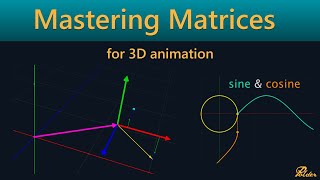
Mastering Matrices for 3D animation
Jean-Paul Tossings
SRT - Most compatible format for video players (VLC, media players, video editors)
VTT - Web Video Text Tracks for HTML5 video and browsers
TXT - Plain text with timestamps for easy reading and editing
Scroll to view all subtitles
hello everyone Jean poing here technical
director at poer animation in my
day-to-day work I use a lot of linear
algebra and matrices are a big part of
that and they can be really powerful in
rigging if used correctly everyone using
a 3D software package uses matrices but
most of the time without knowing it when
moving rotating scaling Andor parenting
objects you are basically modifying
matrices up until a few Maya versions
back matrices could not be used directly
to transform objects X without
decomposing the matrices into separate
translate rotating scale values this
made working with them lose a lot of
power due to unnecessary expensive
calculations but since Maya 2020 The
Matrix workflow has been updated and
since then the full power of matrices
has been unlocked but to use this
workflow to your full advantage you have
to understand what a matrix is and how
it works when I first started working
with them it took me a while to truly
grasp the concept of them and I see the
same struggles with people I work with
that start using them so I decided to do
a video about them trying to explain
matrices in the way that makes sense to
me visually I will start with the basics
and build up to how they work you may
already know the basics but I'll advise
you not to skip ahead because there is a
logical buildup I use Maya as example
for this video but this applies to every
3D
DCC the coordinate system let's start by
defining a three-dimensional coordinate
system system we have three coordinate
axis one for each Dimension all
orthogonal meaning they all form a right
angle with one another we call the point
where all three axes intersect the
origin if we have three coordinates X Y
and Z we can visit any position in this
space by starting at the origin and
moving parallel to the coordinate axis
by the amount of each coordinate this is
known as a cartisian coordinate system
let's call this the root coordinate
space this will be the space where
everything we're going to do will be def
find in points and vectors in this
coordinate system we can create points
and vectors points have a position in
space defined by the coordinates vectors
have a direction and a length a vector
starts at the origin and the tip
position is defined by the coordinates
however vectors can be placed anywhere
in the space as only their Direction and
length matters so placing the vector
root at any point in space we arrive at
the vector T position by moving parallel
to the coordinate axis by the amount of
the
coordinates a vector with a length of
one is called a unit
Vector vectors can be added by placing
them root to tip the resulting Vector
starts at the root of the first vector
and ends at the tip of the last Vector
the order of the vectors does not matter
the resulting Vector will always be the
same for now both points and vectors
have three coordinates and have the same
coordinate
notation 3x3 Matrix
now let's define three new unit vectors
one for each axis and call these the X Y
and Z basis vectors if we scale these
basis vectors by multiplying them with
the corresponding Point coordinates and
add them together we arrive at the
resulting Point position in the same
manner we can arrive at the vector tip
using the vector components because the
basis vectors or unit vectors and are
aligned with the coordinate axis we
arrive at the same positions as when
moving parallel to the root space
coordinate axis let's introduce some
point coordinates and plot them using
the scale basis vectors connecting the
points with edges gives us a cube then
add some vectors in the same manner now
look at what happens if we manipulate
the basis vectors if we change the
length of a basis Vector we scale the
space in that direction all points and
Vector tips get transformed because they
use the scaled version of the basis
Vector to arrive at their positions if
we move prove the tips of the basis
vectors in a circular motion around an
arbitrary line the space and all its
points and vectors inside rotate in the
root coordinate space if we break the
orthogonality of the basis vectors the
space they defined get skewed this is
called
share we can arbitrarily change the
basis vectors to deform the coordinate
space all points and vectors inside it
get transformed with it it is all
relative however the local coordinates
of the points and vectors that live
inside the space do not change only the
space itself gets distorted it is when
looking at them from the outside in the
root space that we see the transformed
coordinates of the points and vectors so
with these three basis vectors we have
to find a new space that we can
transform within the root Space by
adjusting the basis vectors if we look
at the three basis factors as rows they
form the 3X3 Matrix ation of this
transformed space to get the root space
coordinates from the points inside the
Matrix space we multiply the points
local coordinates with its respective
Matrix row and add the scaled rows
together this action is called
multiplying a point with a matrix in
other words when we multiply a point
with a matrix we end up with another
point which has the Matrix
transformation baked into its
coordinates multiplying a vector with a
matrix works the same way
with this 3x3 Matrix we can rotate scale
and share the space and its points and
vectors translation but what about
translation with the current Matrix we
cannot move the space as a whole in
other words we cannot move all points
inside the space while maintaining their
absolute distances in the root
coordinate space to accomplish this we
need to add an extra translation factor
to the sum of scaled basis factors as we
have seen before the order ofor vector
addition does not matter so let's
reorder them to get a more visually
pleasing
representation now you could also
visually interpret the translation
Factor as moving the origin of this
space to a new position if we add the
translation Factor as an extra row to
The Matrix we can add it mathematically
to the sum of scaled basis vectors but
now we need an extra coordinate in the
definition of the points and vectors to
scale the translation Vector with this
is called called The W component now we
have an x y z and W component to
respectively multiply with the basis
Factor XYZ and the translation factor
for points transformed by The Matrix the
translation should always be added 100%
and not a scaled amount so the W
component should always be one for
points vectors however have no use for
translation as they can be positioned
anywhere in space and as we have seen
before the vector coordinates Define the
tip position relative to its root in
other words its direction and length so
adding the translation would only change
the tip position of the vector and does
change the length and or its direction
of the vector this is not what we want
when moving the space as a whole the
vectors in it should not change so we
need to ignore the translation for
vectors this can be done by setting the
W component for all vectors to be zero
we can for visual pleasantry set all
Vector roots to the translated origin of
the space this is all arbitrary however
because we can draw the vectors anywhere
in space as long as their Direction and
length remain the same because the W
component should almost always be one
for points and zero for vectors they are
often omitted when writing the
coordinates but they will always be
added before multiplying with a
matrix the 4x4 Matrix so so to construct
a matrix we need three basis vectors as
coordinate AIS and the fourth Vector as
the translated origin but as we have
just concluded vectors and points need a
fourth W component so this should be
true for the vectors making up the
Matrix as well for the three basis
vectors it is clear that the W component
needs to be zero because they are used
as vectors if the translation Vector
would also get a w component of zero
then when multiplying a point by this
Matrix the point's W component would be
converted from a one to a zero and thus
converts a point into a vector this is
unwanted so to prevent this the
translation Factor should have a w
component of one and is in fact not a
factor but a point in itself this point
is the origin of the space defined by
The
Matrix after adding the W components to
The Matrix notation we arrive at the
final form the 4x4 Matrix this Matrix
has the ability to translate rotate
scale and share the space and its
content if we modify the 44 Matrix so
that the basis vectors are unit vectors
aligned with the root coordinate axis
and the translation is zero in all
directions we get what is called the
identity Matrix this creates a space
that is identical to the root space and
does not transform anything when
multiplying local coordinates with the
rows of the identity Matrix and adding
them together the result result is the
same coordinates thus multiplying a
point or a vector with the identity
Matrix will result in the same point or
vector matrix
multiplication let's define two new 4x4
matrices A and B we place Matrix B
inside the space of Matrix a and add the
points Cube to the space of Matrix B if
we manipulate Matrix a the basis vectors
and origin point of the inner Matrix B
get trans formed and the transformed
basis vectors and the origin point of
Matrix B are used to get to the point
positions of the
cube the transformations of Matrix a and
Matrix B get added together so to speak
the points inside Matrix B are
transformed by the matrices combined to
mathematically combine these matrices we
simply transform the innermost matrix by
the outer Matrix knowing the Matrix is
composed of three vectors vectors and a
point we can transform the inner matrix
by the outer matrix by just multiplying
the three basis vectors and the point of
the inner Matrix with the outer Matrix
resulting in four new rows and thus a
new
Matrix because we multiply the basis
factors and the origin Point components
of the inner Matrix with the rows of the
outer Matrix we speak of matrix
multiplication we end up with a new 4x4
Matrix that describes all
transformations of Matrix a and Matrix B
combined be aware that the order of
multiplication matters for example
imagine one point and two matrices the
point P has coordinates of 0 0 0 the
first Matrix a has a scaled y basis
Vector of length two the second Matrix B
has a translation of one in the positive
y direction multiplying a with B we get
the new Matrix C if we multiply point B
with Matrix C we get a point at 0 1 0 in
the root space however if we swap the
matrices and multiply B with a we get a
different Matrix D if we multiply point
B with Matrix D we get a point at 0 to0
at the root
space without going into too much detail
mathematically the notation of C equals
B * a where B lives inside a is only
valid for row matrices some software
uses column matrices instead where the
vector components are written top to
bottom and the vectors of the Matrix are
placed next to each other in this case
the multiplication order flips and C = A
* B I will continue with row matrices as
Maya uses this notation however be aware
that bifrost in Maya uses colum matrices
for
example transformation hierarchy
if you build a parent child hierarchy
every item in the hierarchy is a matrix
so parenting is just placing the space
of that Matrix in the space of the
parent Matrix the content of the lowest
child gets transformed by The Matrix of
the child and all the matrices of its
parents if we multiply all these
matrices in sequence we get what is
called the world Matrix multiplying by
this world Matrix transforms the local
coordinates of the lowest child's
content directly into the root space
coordinates so if you have a hierarchy
of a b c d the world Matrix is
calculated by multiplying the matrices
from bottom to top D * C * B *
a we refer to coordinates inside the
Matrix as local space the coordinates in
the parent Matrix as parent space and if
that space is the root coordinate system
we call it World space
invers Matrix matrices also have the
nice property that you can calculate its
inverse transformation I won't go into
the details of how that's beyond the
scope of this video but most dccs have
notes or functions to do this the
inverse Matrix can be seen as the
transformation that undos the
transformation of the Matrix where it
was calculated
from so multiplying a matrix with its
own inverse Matrix will result in the
identity Matrix
the inverse Matrix of the inverse Matrix
is the original Matrix so why is this
use for you my think well for example if
you have a point in World space
coordinates and you multiply it with the
inverse of a matrix you get the point
coordinates in local space of set
Matrix or if you have two matrices in
World space A and B if you multiply B
with the inverse Matrix of a you get a
new Matrix C where b = c * a or in other
words if C were a child of Matrix a they
would together produce the same
Transformations as B thus multiplying
Matrix B with the inverse of Matrix a
returns Matrix B in local coordinates
relative to Matrix
a the inverse Matrix is used when
parenting an object if an object is
placed under its parent the space is
placed inside the space of the parent so
the Matrix of the child is Multiplied
with the Matrix of the parent to get the
child's world Matrix because of this
after the parent action the world
transformations of the child's content
would change in general this is unwanted
so to prevent this during a parenting
action the child's world Matrix gets
multiplied with the new parents inverse
World Matrix to get the new local Matrix
relative to the parent the child's
Matrix is then updated to this new local
Matrix and when multiplied with the
parent Matrix the Transformations add up
to the same world Matrix as before the
parent action Maya's parenting operation
does this by default but offers the
relative option to not change the chance
Matrix and thus keep its local Matrix as
is I will use this inverse Matrix to get
the local Matrix extensively in a
follow-up video about flat dynamic
control rigs using
guides composing a matrix all 3D
software packages work with matrices
behind the scenes any object that can be
translated rotated or scaled is
basically a matrix a piece of geometry
for example is just a collection of
points and vectors in local space and
when moving the geometry Only The Matrix
is manipulated the unchanged points and
vectors then get transformed by this
Matrix to get their world positions for
drawing them on screen in Maya all
geometry Point data is stored in the
shape node which is a child of a
transform node the shape node has no
Matrix data but the transform node
stores The Matrix however most of the
time the user gets presented with
individual translate rotate and scale
values because directly manipulating a
matrix is not very intuitive when
changing these translation rotation in
scale values to modify an object behind
the scenes a matrix is composed to
transform the object's points vectors
and or child matrices in fact in the
transformation node not one Matrix is
composed but multiple one for
translation three for rotation one for
scale one for share a few for rotation
and scale pivot offsets and one parent
offset Matrix a joint even has an
additional three matrices for the joint
Orient and an extra inverse Scale Matrix
all these matrices get multiply together
in the way I showed earlier in a
specific order to form the final
transformation matrix of the transform
node you could look at this as a whole
hierarchy of matrices inside the
transform node all of these internal
matrices are composed from the values
set on the transform node the basis or
template if you will of all these
individual matrices is always the
identity Matrix now let's look at how to
modify these identity matrices to get
translate rotate scale and share
matrices translation the translation
Matrix can be created by setting the
values directly as the X Y and Z values
of the translation
Vector scale the Scale Matrix can be
created by scaling the basis vectors by
its corresponding scale value but as
these are unit factors in the identity
Matrix we can set them directly to the
value that has
D1 rotation for rotation usually in
Oiler rotation is used where you specify
three rotation values for rotating
around the X Y and Z axis respectively
each value is used to create a separate
Matrix that is rotated by the amount
around the axis all three matrices are
then multiplied together to get the
complete rotation Matrix this is why we
also have a rotation order for this
rotation this determines the order in
which the X Y and Z rotation matrices
are multiplied each combination gives a
different result because the
multiplication order matters for
matrices before creating the three
rotation matrices we first need to take
a look at the S and cosine function the
S and cosine functions Loop every 2 pi
which corresponds with one unit circle
circumference if we rotate the cosine
graph 90° we can use the cosine and S
values as 2D coordinates to trace a
circle with a radius of one the input of
the sign and cosine can now be seen as a
rotation in Radiance of a unit Vector
with coordinates 1
Z because the basis vectors of the
identity Matrix are unit vectors and the
combined s and cosine values also create
a unit Vector we can create any angled
basis vector by using the S and cosine
of the angle in radians as two
components of the basis
vectors to get the rotation xate
we rotate the Y and Z basis factors
around the X basis
Vector so the X basis Vector does not
change and because the rotation happens
in the y z axis plane the X components
of the Y and Z basis vectors also do not
change we can discard the X Dimension
and look at the Y and Z as components of
a 2d Vector this is where the sign and
cosine come in with a rotation of zero
the cosine evaluates to one and the S
evaluates to zero so we can just
substitute the ones with cosine of angle
and the Zer with s of angle the Y basis
Factor thus becomes zero cosine of angle
s of angle the Z basis Factor becomes
zero s of angle cosine of angle because
the sign and cosine needs angles in
radians and the user enters Oiler angles
in degrees internally the the user
angles are converted to radians by
dividing them by 2 pi however when we
now rotate the basis factors by setting
an angle other than zero the bases X's
do not rotate in the same direction so
we have to flip the direction of one of
the components by negating it we cannot
negate a cosine because it is one at
zero rotation and that would flip the
basis Factor the sign is zero at a
rotation of zero so negating that does
not change the not rotated basis Factor
the direction of rotation is based as
far as I know on the following
convention when you align the thumb of
your hand with the x-axis your index
finger with the Y AIS and your middle
finger with the z-axis this can only
match with either your left or your
right hand the coordinate system is thus
said to be right-handed or left-handed
when you take the hand that matches and
make a thumbs up sign and align the
thumb with the positive direction of the
axis you are rotating around for fingers
Arc in the direction of positive
rotation so for a right-handed
coordinate system positive rotation is
always
counterclockwise taking this into
account we have to negate the sign of
angle in the Z basis Vector following
the same logic we end up with a Y
rotation Matrix with a negated sign of
angle in the X basis vector and the Z
rotation Matrix with a negated sign of
angle in the Y basis Vector multiplying
these three rotation matrices in the
specify rotation order results in the
full rotation
Matrix
share in general Shear is not something
that a user would manually set but it's
usually exposed to the user to
manipulate the transformation matrix
there are different ways of implementing
Shear in a matrix in Maya the sheare
values are set directly at the following
positions to introduce the slanted
axis so now you hopefully have a better
understanding of matrices and the way to
visualize what is happening I know this
helped me a lot with the mystifying
matrices when I started working with
them there is still more to discover
like creating a rotation Matrix from a
querian instead of oil rotation or how
to decompose a matrix in its separate
Transformations if you're interested in
this leave a comment and maybe I'll
create a follow-up video I'll also be
doing some practical example videos of
working with matrices so stay tuned
follow And subscribe and let me know in
the comments what you think of the
content
Full transcript without timestamps
hello everyone Jean poing here technical director at poer animation in my day-to-day work I use a lot of linear algebra and matrices are a big part of that and they can be really powerful in rigging if used correctly everyone using a 3D software package uses matrices but most of the time without knowing it when moving rotating scaling Andor parenting objects you are basically modifying matrices up until a few Maya versions back matrices could not be used directly to transform objects X without decomposing the matrices into separate translate rotating scale values this made working with them lose a lot of power due to unnecessary expensive calculations but since Maya 2020 The Matrix workflow has been updated and since then the full power of matrices has been unlocked but to use this workflow to your full advantage you have to understand what a matrix is and how it works when I first started working with them it took me a while to truly grasp the concept of them and I see the same struggles with people I work with that start using them so I decided to do a video about them trying to explain matrices in the way that makes sense to me visually I will start with the basics and build up to how they work you may already know the basics but I'll advise you not to skip ahead because there is a logical buildup I use Maya as example for this video but this applies to every 3D DCC the coordinate system let's start by defining a three-dimensional coordinate system system we have three coordinate axis one for each Dimension all orthogonal meaning they all form a right angle with one another we call the point where all three axes intersect the origin if we have three coordinates X Y and Z we can visit any position in this space by starting at the origin and moving parallel to the coordinate axis by the amount of each coordinate this is known as a cartisian coordinate system let's call this the root coordinate space this will be the space where everything we're going to do will be def find in points and vectors in this coordinate system we can create points and vectors points have a position in space defined by the coordinates vectors have a direction and a length a vector starts at the origin and the tip position is defined by the coordinates however vectors can be placed anywhere in the space as only their Direction and length matters so placing the vector root at any point in space we arrive at the vector T position by moving parallel to the coordinate axis by the amount of the coordinates a vector with a length of one is called a unit Vector vectors can be added by placing them root to tip the resulting Vector starts at the root of the first vector and ends at the tip of the last Vector the order of the vectors does not matter the resulting Vector will always be the same for now both points and vectors have three coordinates and have the same coordinate notation 3x3 Matrix now let's define three new unit vectors one for each axis and call these the X Y and Z basis vectors if we scale these basis vectors by multiplying them with the corresponding Point coordinates and add them together we arrive at the resulting Point position in the same manner we can arrive at the vector tip using the vector components because the basis vectors or unit vectors and are aligned with the coordinate axis we arrive at the same positions as when moving parallel to the root space coordinate axis let's introduce some point coordinates and plot them using the scale basis vectors connecting the points with edges gives us a cube then add some vectors in the same manner now look at what happens if we manipulate the basis vectors if we change the length of a basis Vector we scale the space in that direction all points and Vector tips get transformed because they use the scaled version of the basis Vector to arrive at their positions if we move prove the tips of the basis vectors in a circular motion around an arbitrary line the space and all its points and vectors inside rotate in the root coordinate space if we break the orthogonality of the basis vectors the space they defined get skewed this is called share we can arbitrarily change the basis vectors to deform the coordinate space all points and vectors inside it get transformed with it it is all relative however the local coordinates of the points and vectors that live inside the space do not change only the space itself gets distorted it is when looking at them from the outside in the root space that we see the transformed coordinates of the points and vectors so with these three basis vectors we have to find a new space that we can transform within the root Space by adjusting the basis vectors if we look at the three basis factors as rows they form the 3X3 Matrix ation of this transformed space to get the root space coordinates from the points inside the Matrix space we multiply the points local coordinates with its respective Matrix row and add the scaled rows together this action is called multiplying a point with a matrix in other words when we multiply a point with a matrix we end up with another point which has the Matrix transformation baked into its coordinates multiplying a vector with a matrix works the same way with this 3x3 Matrix we can rotate scale and share the space and its points and vectors translation but what about translation with the current Matrix we cannot move the space as a whole in other words we cannot move all points inside the space while maintaining their absolute distances in the root coordinate space to accomplish this we need to add an extra translation factor to the sum of scaled basis factors as we have seen before the order ofor vector addition does not matter so let's reorder them to get a more visually pleasing representation now you could also visually interpret the translation Factor as moving the origin of this space to a new position if we add the translation Factor as an extra row to The Matrix we can add it mathematically to the sum of scaled basis vectors but now we need an extra coordinate in the definition of the points and vectors to scale the translation Vector with this is called called The W component now we have an x y z and W component to respectively multiply with the basis Factor XYZ and the translation factor for points transformed by The Matrix the translation should always be added 100% and not a scaled amount so the W component should always be one for points vectors however have no use for translation as they can be positioned anywhere in space and as we have seen before the vector coordinates Define the tip position relative to its root in other words its direction and length so adding the translation would only change the tip position of the vector and does change the length and or its direction of the vector this is not what we want when moving the space as a whole the vectors in it should not change so we need to ignore the translation for vectors this can be done by setting the W component for all vectors to be zero we can for visual pleasantry set all Vector roots to the translated origin of the space this is all arbitrary however because we can draw the vectors anywhere in space as long as their Direction and length remain the same because the W component should almost always be one for points and zero for vectors they are often omitted when writing the coordinates but they will always be added before multiplying with a matrix the 4x4 Matrix so so to construct a matrix we need three basis vectors as coordinate AIS and the fourth Vector as the translated origin but as we have just concluded vectors and points need a fourth W component so this should be true for the vectors making up the Matrix as well for the three basis vectors it is clear that the W component needs to be zero because they are used as vectors if the translation Vector would also get a w component of zero then when multiplying a point by this Matrix the point's W component would be converted from a one to a zero and thus converts a point into a vector this is unwanted so to prevent this the translation Factor should have a w component of one and is in fact not a factor but a point in itself this point is the origin of the space defined by The Matrix after adding the W components to The Matrix notation we arrive at the final form the 4x4 Matrix this Matrix has the ability to translate rotate scale and share the space and its content if we modify the 44 Matrix so that the basis vectors are unit vectors aligned with the root coordinate axis and the translation is zero in all directions we get what is called the identity Matrix this creates a space that is identical to the root space and does not transform anything when multiplying local coordinates with the rows of the identity Matrix and adding them together the result result is the same coordinates thus multiplying a point or a vector with the identity Matrix will result in the same point or vector matrix multiplication let's define two new 4x4 matrices A and B we place Matrix B inside the space of Matrix a and add the points Cube to the space of Matrix B if we manipulate Matrix a the basis vectors and origin point of the inner Matrix B get trans formed and the transformed basis vectors and the origin point of Matrix B are used to get to the point positions of the cube the transformations of Matrix a and Matrix B get added together so to speak the points inside Matrix B are transformed by the matrices combined to mathematically combine these matrices we simply transform the innermost matrix by the outer Matrix knowing the Matrix is composed of three vectors vectors and a point we can transform the inner matrix by the outer matrix by just multiplying the three basis vectors and the point of the inner Matrix with the outer Matrix resulting in four new rows and thus a new Matrix because we multiply the basis factors and the origin Point components of the inner Matrix with the rows of the outer Matrix we speak of matrix multiplication we end up with a new 4x4 Matrix that describes all transformations of Matrix a and Matrix B combined be aware that the order of multiplication matters for example imagine one point and two matrices the point P has coordinates of 0 0 0 the first Matrix a has a scaled y basis Vector of length two the second Matrix B has a translation of one in the positive y direction multiplying a with B we get the new Matrix C if we multiply point B with Matrix C we get a point at 0 1 0 in the root space however if we swap the matrices and multiply B with a we get a different Matrix D if we multiply point B with Matrix D we get a point at 0 to0 at the root space without going into too much detail mathematically the notation of C equals B * a where B lives inside a is only valid for row matrices some software uses column matrices instead where the vector components are written top to bottom and the vectors of the Matrix are placed next to each other in this case the multiplication order flips and C = A * B I will continue with row matrices as Maya uses this notation however be aware that bifrost in Maya uses colum matrices for example transformation hierarchy if you build a parent child hierarchy every item in the hierarchy is a matrix so parenting is just placing the space of that Matrix in the space of the parent Matrix the content of the lowest child gets transformed by The Matrix of the child and all the matrices of its parents if we multiply all these matrices in sequence we get what is called the world Matrix multiplying by this world Matrix transforms the local coordinates of the lowest child's content directly into the root space coordinates so if you have a hierarchy of a b c d the world Matrix is calculated by multiplying the matrices from bottom to top D * C * B * a we refer to coordinates inside the Matrix as local space the coordinates in the parent Matrix as parent space and if that space is the root coordinate system we call it World space invers Matrix matrices also have the nice property that you can calculate its inverse transformation I won't go into the details of how that's beyond the scope of this video but most dccs have notes or functions to do this the inverse Matrix can be seen as the transformation that undos the transformation of the Matrix where it was calculated from so multiplying a matrix with its own inverse Matrix will result in the identity Matrix the inverse Matrix of the inverse Matrix is the original Matrix so why is this use for you my think well for example if you have a point in World space coordinates and you multiply it with the inverse of a matrix you get the point coordinates in local space of set Matrix or if you have two matrices in World space A and B if you multiply B with the inverse Matrix of a you get a new Matrix C where b = c * a or in other words if C were a child of Matrix a they would together produce the same Transformations as B thus multiplying Matrix B with the inverse of Matrix a returns Matrix B in local coordinates relative to Matrix a the inverse Matrix is used when parenting an object if an object is placed under its parent the space is placed inside the space of the parent so the Matrix of the child is Multiplied with the Matrix of the parent to get the child's world Matrix because of this after the parent action the world transformations of the child's content would change in general this is unwanted so to prevent this during a parenting action the child's world Matrix gets multiplied with the new parents inverse World Matrix to get the new local Matrix relative to the parent the child's Matrix is then updated to this new local Matrix and when multiplied with the parent Matrix the Transformations add up to the same world Matrix as before the parent action Maya's parenting operation does this by default but offers the relative option to not change the chance Matrix and thus keep its local Matrix as is I will use this inverse Matrix to get the local Matrix extensively in a follow-up video about flat dynamic control rigs using guides composing a matrix all 3D software packages work with matrices behind the scenes any object that can be translated rotated or scaled is basically a matrix a piece of geometry for example is just a collection of points and vectors in local space and when moving the geometry Only The Matrix is manipulated the unchanged points and vectors then get transformed by this Matrix to get their world positions for drawing them on screen in Maya all geometry Point data is stored in the shape node which is a child of a transform node the shape node has no Matrix data but the transform node stores The Matrix however most of the time the user gets presented with individual translate rotate and scale values because directly manipulating a matrix is not very intuitive when changing these translation rotation in scale values to modify an object behind the scenes a matrix is composed to transform the object's points vectors and or child matrices in fact in the transformation node not one Matrix is composed but multiple one for translation three for rotation one for scale one for share a few for rotation and scale pivot offsets and one parent offset Matrix a joint even has an additional three matrices for the joint Orient and an extra inverse Scale Matrix all these matrices get multiply together in the way I showed earlier in a specific order to form the final transformation matrix of the transform node you could look at this as a whole hierarchy of matrices inside the transform node all of these internal matrices are composed from the values set on the transform node the basis or template if you will of all these individual matrices is always the identity Matrix now let's look at how to modify these identity matrices to get translate rotate scale and share matrices translation the translation Matrix can be created by setting the values directly as the X Y and Z values of the translation Vector scale the Scale Matrix can be created by scaling the basis vectors by its corresponding scale value but as these are unit factors in the identity Matrix we can set them directly to the value that has D1 rotation for rotation usually in Oiler rotation is used where you specify three rotation values for rotating around the X Y and Z axis respectively each value is used to create a separate Matrix that is rotated by the amount around the axis all three matrices are then multiplied together to get the complete rotation Matrix this is why we also have a rotation order for this rotation this determines the order in which the X Y and Z rotation matrices are multiplied each combination gives a different result because the multiplication order matters for matrices before creating the three rotation matrices we first need to take a look at the S and cosine function the S and cosine functions Loop every 2 pi which corresponds with one unit circle circumference if we rotate the cosine graph 90° we can use the cosine and S values as 2D coordinates to trace a circle with a radius of one the input of the sign and cosine can now be seen as a rotation in Radiance of a unit Vector with coordinates 1 Z because the basis vectors of the identity Matrix are unit vectors and the combined s and cosine values also create a unit Vector we can create any angled basis vector by using the S and cosine of the angle in radians as two components of the basis vectors to get the rotation xate we rotate the Y and Z basis factors around the X basis Vector so the X basis Vector does not change and because the rotation happens in the y z axis plane the X components of the Y and Z basis vectors also do not change we can discard the X Dimension and look at the Y and Z as components of a 2d Vector this is where the sign and cosine come in with a rotation of zero the cosine evaluates to one and the S evaluates to zero so we can just substitute the ones with cosine of angle and the Zer with s of angle the Y basis Factor thus becomes zero cosine of angle s of angle the Z basis Factor becomes zero s of angle cosine of angle because the sign and cosine needs angles in radians and the user enters Oiler angles in degrees internally the the user angles are converted to radians by dividing them by 2 pi however when we now rotate the basis factors by setting an angle other than zero the bases X's do not rotate in the same direction so we have to flip the direction of one of the components by negating it we cannot negate a cosine because it is one at zero rotation and that would flip the basis Factor the sign is zero at a rotation of zero so negating that does not change the not rotated basis Factor the direction of rotation is based as far as I know on the following convention when you align the thumb of your hand with the x-axis your index finger with the Y AIS and your middle finger with the z-axis this can only match with either your left or your right hand the coordinate system is thus said to be right-handed or left-handed when you take the hand that matches and make a thumbs up sign and align the thumb with the positive direction of the axis you are rotating around for fingers Arc in the direction of positive rotation so for a right-handed coordinate system positive rotation is always counterclockwise taking this into account we have to negate the sign of angle in the Z basis Vector following the same logic we end up with a Y rotation Matrix with a negated sign of angle in the X basis vector and the Z rotation Matrix with a negated sign of angle in the Y basis Vector multiplying these three rotation matrices in the specify rotation order results in the full rotation Matrix share in general Shear is not something that a user would manually set but it's usually exposed to the user to manipulate the transformation matrix there are different ways of implementing Shear in a matrix in Maya the sheare values are set directly at the following positions to introduce the slanted axis so now you hopefully have a better understanding of matrices and the way to visualize what is happening I know this helped me a lot with the mystifying matrices when I started working with them there is still more to discover like creating a rotation Matrix from a querian instead of oil rotation or how to decompose a matrix in its separate Transformations if you're interested in this leave a comment and maybe I'll create a follow-up video I'll also be doing some practical example videos of working with matrices so stay tuned follow And subscribe and let me know in the comments what you think of the content
Download Subtitles
These subtitles were extracted using the Free YouTube Subtitle Downloader by LunaNotes.
Download more subtitlesRelated Videos
Download Subtitles for Rigging with Matrices - Part 02 FK Tutorial
Enhance your learning experience with downloadable subtitles for the 'Rigging with Matrices - Part 02 FK' video. Subtitles provide clear guidance, making complex rigging techniques easier to understand and follow along. Perfect for students and 3D animation enthusiasts wanting detailed explanations in text form.

Download Subtitles for Introduction to DaVinci Resolve Full Course
Enhance your learning experience by downloading accurate subtitles for the Introduction to DaVinci Resolve full course. Captions help you follow along effortlessly, improve comprehension, and make the tutorial accessible anytime, anywhere.

Download Subtitles for 140 Soft Acrobatics Moves Tutorial
Enhance your learning experience by downloading accurate subtitles for the '140 Soft Acrobatics Moves Adult Beginners Can Actually Master' video. Subtitles help you follow instructions clearly, improve understanding, and practice safely at your own pace.
Download Subtitles for All Machine Learning Concepts Video
Enhance your understanding by downloading accurate subtitles for the 'All Machine Learning Concepts Explained in 22 Minutes' video. Access clear captions to follow complex topics with ease and improve your learning experience.

Download Subtitles for The Guillotine Choke Masterclass Video
Enhance your learning experience with downloadable subtitles for The Guillotine Choke: A Complete Masterclass. Perfect for following along, improving comprehension, and mastering every technique showcased in this instructional video.
Most Viewed

Untertitel für 'Nicos Weg' Deutsch lernen A1 Film herunterladen
Laden Sie die Untertitel für den gesamten Film 'Nicos Weg' herunter, um Ihr Deutschlernen auf A1 Niveau zu unterstützen. Untertitel helfen Ihnen, Wortschatz und Aussprache besser zu verstehen und verbessern das Hörverständnis effektiv.

ดาวน์โหลดซับไตเติ้ล DMD LAND 3 The Final Land Day 1
ดาวน์โหลดซับไตเติ้ลสำหรับวิดีโอ DMD LAND 3 The Final Land Day 1 เพื่อช่วยให้เข้าใจเนื้อหาได้ง่ายขึ้น และเพิ่มความสะดวกในการติดตามทุกช่วงเวลา เหมาะสำหรับผู้ชมที่ต้องการความชัดเจนและเข้าถึงข้อมูลอย่างครบถ้วน

Descarga Subtítulos para NARCISISMO | 6 DE COPAS - Episodio 63
Accede fácilmente a los subtítulos del episodio 63 de '6 DE COPAS', centrado en el narcisismo. Descargar estos subtítulos te ayudará a entender mejor el contenido y mejorar la experiencia de visualización.

Subtítulos para TIPOS DE APEGO | 6 DE COPAS Episodio 56
Descarga los subtítulos para el episodio 56 de la tercera temporada de 6 DE COPAS, centrado en los tipos de apego. Mejora tu comprensión y disfruta del contenido en detalle con nuestros subtítulos precisos y accesibles.

Download Subtitles for Your Favorite Videos Easily
Enhance your video watching experience by downloading accurate subtitles and captions. Enjoy better understanding, accessibility, and language support for all your favorite videos.

If you found these subtitles useful, consider buying us a coffee. It would help us a lot!