Introduction to Linear Transformations in Machine Learning
Matrix multiplication is fundamental in machine learning, representing linear transformations that map input vectors to output vectors in geometric space. Understanding this concept strengthens your foundation in linear algebra. For a broader foundational understanding, consider reviewing Linear Algebra Foundations for Machine Learning: Vectors, Span, and Basis Explained.
What is a Transformation?
- A transformation changes an input vector into an output vector.
- Visualized in 2D space with vectors originating at the origin.
Properties of Linear Transformations
- Preservation of Lines: All points originally on a straight line remain on a straight line after transformation.
- Fixed Origin: The origin (0,0) does not move under transformation.
Examples:
- Case 1: Input vector tips on a line remain on a line; origin fixed. This defines a linear transformation.
- Case 2: Output vector tips do not lie on a straight line; origin fixed. Not a linear transformation.
- Case 3: Vector tips remain on a line but origin shifts. Not a linear transformation.
Representing Vectors and Transformations
- Any 2D vector v can be expressed as a linear combination: v = xI + yJ, where I and J are basis vectors.
- A linear transformation can be understood by observing how I and J themselves are transformed.
Transformation Example: Rotation + Scaling
- Rotate vectors by 90° counterclockwise and scale by 2.
- The transformed vector U = 1 * (Transformed I) + 2 * (Transformed J).
- By knowing the transformed basis vectors, the transformation on any vector can be deduced.
Matrix Representation of Transformations
- Transformation matrix columns correspond to transformed basis vectors:
- First column = transformed I
- Second column = transformed J
- Applying this matrix to vector coordinates implements the transformation:
U = \begin{bmatrix} a & b \ c & d \end{bmatrix} \begin{bmatrix} x \ y \end{bmatrix} = x(a,c) + y(b,d) \ - This connects the geometric intuition of transformations to matrix multiplication.
Common Linear Transformations and Their Matrices
- 90° Counterclockwise Rotation:
\begin{bmatrix} 0 & -1 \ 1 & 0 \end{bmatrix} \ - Shear Transformation:
- I remains unchanged, J moves to (1,1)
\begin{bmatrix} 1 & 1 \ 0 & 1 \end{bmatrix} \
- I remains unchanged, J moves to (1,1)
- Squishing to One Dimensional Line:
- I and J become parallel vectors
\begin{bmatrix} 1 & -1 \ 1 & -1 \end{bmatrix} \ - Results in loss of linear independence, determinant zero
- I and J become parallel vectors
Key Insights
- Linear transformations rely solely on how basis vectors transform.
- Matrix multiplication is a compact representation of these transformations.
- Understanding basis vector transformations allows intuitive comprehension of matrix actions on vectors.
- Determinant zero transformations compress dimensions, reducing space spanned.
Conclusion
By interpreting matrix multiplication as linear transformations acting on basis vectors, we gain powerful geometric intuition essential for machine learning and linear algebra. This approach simplifies understanding rotations, shearing, scaling, and more complex transformations in 2D vector spaces.
For further insights on the mechanics behind these concepts, exploring Understanding Elementary Row Operations in Matrix Analysis can be highly beneficial. Additionally, to see practical applications of such linear transformations in machine learning, review Understanding Linear Classifiers in Image Classification.
[Music] hi welcome to a new lecture from the course foundations for machine learning
we are learning about linear algebra and specifically in this lecture we'll be looking at Matrix
multiplications what we are trying to understand in this lecture is the intuition that matrix multiplication is
essentially a linear transformation so we'll see how that happens how vectors are transformed in a linear fashion when
you multiply them with matrices this is an operation that is commonly seen across machine learning so if you have a
fairly good geometric or intuitive understanding of this whole idea it makes your foundations very very strong
so let us start with what do we mean by a transformation a transformation is
nothing but something that changes an input Vector to an output Vector so here I have drawn a 2d Space X Y and I have a
vector V1 and Vector V2 and a transformation is defined as you can think of it as a function f which
transforms the vector V1 into vs2 so please note that in this lecture I'm not strictly following the convention of
what should be input vector and what should be output Vector uh as in I may be using the notation U or V uh
interchangeably for input or output but wherever it's the whereever ever I'm using v as the input vector or U as the
output Vector I'll be very clearly defining what is input and what is output so please don't get confused uh
if uh you know if I'm not sticking with certain notations that you may be familiar with so a transformation is
nothing but something that changes a vector into something else so here we see that the vector is still in the 2D
space after transformation but it has uh it's you know the head or its tip rather it has mov
now there are several types of Transformations but specifically we are trying to learn about linear
transformation and this is probably the the Cornerstone of linear algebra if there is one concept that you should
absolutely master in linear algebra it is definitely linear Transformations linear transformation
has two properties as I have written here all straight lines must remain as straight lines
this is the first property in a linear transformation the second property is that the origin should not move the
origin should remain fixed now let us see what the first point specifically means when I say
origin should not move I I'm pretty sure that you can imagine that really well but when I say all lines might must
remain as lines I'm not really certain that you are Imagining the exact same thing that you are supposed to imagine
so what lines are we talking about here let's start with an example right so let's visualize a particular
transformation some of these transformation may be linear some of them may be uh not linear but let's see
so here imagine you have three vectors that are inputs into the transformation V1 V2 V3 and you have two uh three
vectors that are outputs U1 U2 and u3 um my question is is this a linear transformation or
not one of the ways to see whether this is a linear transformation or not is to check if the the two properties
above uh all lines must remain lines origin should not move whether these two conditions are satisfied or not now you
might be wondering that oh the vector looks like a straight line so this is a linear transformation because the lines
are remaining as Lines no that is not what we mean by the lines here because there are no vectors like this if you if
you have something like this this is not a vector right there is no Vector that looks like this so obviously all the
vectors are going to look like straight lines only so we are not talking about that straight line so what are we
actually talking about we are talking about the line formed by the tips of vectors so imagine that these three
vectors are these are these are three points that represent the coordinates of the tips of the vectors so I'm when I
say tip I mean the head of the vector and tail is this so tail is the back back end of the vector tip is the head
end of the vector so here these three points are essentially on the straight on a straight line right now you can
imagine that uh V1 V2 V3 have uh three corresponding coordinates which correspond to the head of these vectors
now let's see what happens to those coordinates after transformation so after transformation V1 becomes U one so
now the new new tip is this V2 becomes U2 so the new tip is this V3 becomes u3 so the new tip is this and you can see
that the modified tips are also on a straight line so this straight line got transformed into this straight line so
the lines are staying as lines and on top of that the origin has not moved the transform vectors as well as the input
vectors have the same origin uh which is 0 0 on the coordinate system so in this case
one we can see that this is essentially a linear transformation now let's look at another
Case Case two in case two we have again the same three input vectors so we can Define the
the three coordinate points uh which form the tip of these vectors right so these three points we
can see that they are on a straight line but now the let's look at the transformed vectors U1 U2 and u3 so the
U1 has tip here U2 has a tip here and u3 has a tip here so we can see that the the points of the points that form the
head of these three vectors after transformation they do not lie on a straight line so the straight line over
here got transformed into something that is not a straight line because we cannot draw a line between this point this
point Point like you know this point this point and this point do not lie on a straight line but the origin is
still you know intact the input vectors have 0 0 as the origin and outputs also have 0 0 as the origin so here in the
linear transformation among the two conditions the second condition was satisfied in this case to but the first
condition all lines must remain lines it was not satisfied so this is not a linear transformation example in case
two case one this was a linear transformation but case two this is not a linear
transformation let us look at one more case here you have three vectors V1 vs2 V3 and imagine they are transformed into
U1 U2 u3 is this a linear transformation the the tips are in a straight line over
here so these tips of in input vectors were in a straight line the tips of the output vectors
are also in a straight line however this is not a linear transformation because the the tail of
these vectors are now no more at the origin so the origin has sort of shifted from0 Z to something else so in case
three this is also not a linear transformation but case one was a linear transformation because the straight
lines remained as a straight line the origin was was unaffected by the transformation so this is how we should
visualize linear transformation so always visualize where the tips of the vectors are moving whenever a
transformation is happening and by tracking those tips we can track whether straight lines remain as straight lines
or not so now let us see how to numerically
describe some of these Transformations because so far we have been describing it a bit qualitatively
so take an example of a vector let's say vector v uh in XY plane like this V is described in this specific example as I
+ 2J because on the x- axis the dimension is 1 along the y- axis it is 2 so the vector v is defined as 1 I + 2 J
and you should remember what this is this is scaling plus linear combination of the two basis vectors I and J are the
basis vectors here right and you can express any Vector in the XY coordinate system using these basis vectors and I
and J are probably the most fundamental basis vectors that any student learns first and you can represent this vector
v in terms of the scaling so what do we mean by scaling here we multiply by a scalar so here the the scalar number
using which the vector I is Multiplied is one the scalar number by which Vector J is Multiplied is two and why do we say
linear combination because we are directly adding those two vectors so V is defined as the scaling plus linear
combination of I and J and I and J are the basis vectors so this sounds trivial right so why am I mentioning this I'm
mentioning this because I also want to show you how this same principle applies after we do the transformation on top of
vector v so let us Define a very simple transformation um let's say the transformation involves two steps first
is rotation by 90° counterclockwise so whatever Vector is present in the in this transformation it will be rotated
by 90° counterclockwise and uh also as part of the transformation the same Vector will
be simultaneously scaled up by a factor of two so the size of the vector doubles but the vector itself will get rotated
by 90° so we can see what happens to this particular Vector under such a
transformation so the original vector v this will be rotated by 90° uh counterclockwise in the counterclockwise
Direction so this is 90° but will the vector remain like this no right because it has to scale up the scaling factor is
two so let me duplicate this Vector something like this and this so now this is the
transformation of the vector v so let me write this as transformed V which one this long guy not this guy
so I'll delete the the the smaller Vector perhaps
okay so now this is the transformed V so you can see the two steps that that happened 90° rotation in
counterclockwise Direction and scaling by a factor of two so
now what we did right now is we we tracked what happened to V similarly can we can we keep track of what happens to
I and J so we said we have to scale uh we have to rotate by 90° clockwise and scale counterclockwise and scale by a
factor of two right so what will happen happen to J J should also be rotated by U 90° counterclockwise and scaled so so
J the origin will remain here but it will it will become this after transformation I can increase the
thickness so that you can see better so this is the transformed J let me write it over
here so this is the transformed J right and what will happen
to I during this transformation I can duplicate I I will be rotated by 90° and scale by a factor of two I can increase
the thickness so this is the transformed I transformed
I this guy so now let us formally represent the vector v once again in terms of uh the
transformed I and transform J but before that let's let's just write this down what happened to I I just want to erase
some of these things so that uh you're not able to see this um let me move this out of your site
I'll come back to I'll come back to you to explain um the transformation that is happening to vector v in terms of
transformation that happened to Vector I and transformation that happened to Vector
J so we saw that V is defined by the linear combin scaling plus linear
combination of I and J right so V was nothing but V was nothing
but um one * I so the here the scaling factor for I is
1 and 2 * J scaling factor for J is two and then we are doing a linear combination of
these scaled I and J vectors and what is V prime or transformed V uh this
transform V I can also denote as V prime or U also uh whatever is convenient for you so maybe I denote it as U um the
transformed V I will call as U so U equal to um just tell me what what does U look
like U looks like two times transform J right two * transform
J maybe transform J I can write as JT so this is J transformed uh transformed I I can
denote as it t I'm sure some of these notations are probably um used in some other context
but I'm not I'm not referring to any of those context I just want to keep it um to the to the geometric intuition at
this point so you can see that the transform V equal to 2 * transform J so that will be this Plus 1 * transformed V
sorry transformed I plus 1 time transformed I I transformed right now here is where
the things get interesting so I can I can write this in the correct order this is 1 * I
transformed plus 2 * J transformed um so this one you saw visually because
visually you can see that this this red Vector which is the transformation is two times this guy uh I need the yellow
Vector two times and I need the green Vector once this green vector and if I add this plus
this I can get the transformed uh V so that is how I wrote it as 2 * J transformed plus 1 * I transformed and
then I flip the order I make it such that uh this 1 * I transformed is coming in the beginning like uh it's it's
written in the beginning and two times J transformed is return second now what do you see the you can see that the
original vector v was 1 * I + 2 * J the transformed vector v which we call as U is again 1 * transformation of I plus 2
* transformation of J so that is what I have written here if V is defined by scal plus linear combination of I and J
then V1 or V transformed whatever you call it V transformed or U is defined by the same scaling Factor so that's why I
have written this word extra the same scaling plus linear combination of i1 and J1 or rather I transformed it and J
transformed JT so that is what we saw here visually we can also prove the same thing numerically very easily but
because uh what happens to I in this case I has transformed to become the coordinate of the I will uh the
coordinate of the tip of the I will be 0 comma 2 right uh the x coordinate will be zero y coordinate will be two so
basically this will be the new this is the position where the I uh I moves to so I will transform to
this guy what happens to J J will transform to um this guy J is scaled by a factor of two
and rotated by 90° counterclockwise so J will have min-2 as its x coordinate after transformation and zero as the
y-coordinate after transformation so this I can also write as in in my previous coordinate system I is
essentially becoming 2J similar to 2J and J is like becoming minus 2 I right so I became 2J and J which was this
Vector it became Min - 2 I so I transforming to this J transforming to this and what is
now the the new transform Vector the new transform Vector will also follow the same thing 1 * whatever is the
transformation of I plus two * whatever is the transformation of J so that is 1 * whatever is the transformation of I
transformation of I is 2J plus 2 * whatever is the transformation
of J 2 * transformation of J is minus 2 i - 2 I so this will be 2 J - 4 I and this can be written in the proper order
as - 4 I + 2J is is this what the new Vector looks like so this is the vector U or V
transformed uh is are minus 4 and two the coordinates of the new Vector let us see in the figure so the new Vector was
this big red guy its x coordinate was Min -4 and y coordinate was 2 so this this the coordinate of this
tip is defined by -4a 2 right and that is exactly what we have got here Min -4 and 2 so this shows uh very intuitively
that if we are performing a linear combination to know where a vector v
will transform and what it will become all we need to know is first see what will happen to
I then see what what will happen to J and if the original vector v by was defined by a certain scaling and linear
combination of I and J all we need to do is perform the same scaling plus linear combination of the transformed I and
transform J so all need to keep track of is what happens to I and what happens to J that's all we don't need to know
anything else so I just want to show you that um uh over here but before that um let's just formally write it down if we
if we know where I and J lands right after the transformation then we will know where
any vector v lands after transformation so if I and J gets rotated by 90° just that if that is the
only thing that happens to the um to the basis vectors I and J then we can know that any vector v will also undergo this
exact same transformation and if I and J becomes i1 and J1 then all we need to do is keep
track of that transmission see what happens to I and J and just apply the same scaling Factor whatever I and J
originally had to the transformed I and transformed J so basically any linear transformation applied on v um that can
change the vector v in such that it will it will be a linear combination of transformed I and transformed J and the
scaling Factor will be remain the same so transformed I will be multiplied by 1 the original I was multiplied by 1
transform J will be multiplied by two original J was multiplied by two uh this is a
fairly uh interesting idea it is it is simple but I don't think many people think of linear transformations in this
way most people think of it as um a complex operation that you have to apply On Any Given random Vector but
you don't have to think of it like that you can think of it as transformation of basis vectors now let's generalize this
just take a general Vector uh V = to x i + YJ which can be written like this right uh X is the uh in vector format we
write like this but if we had written like X comma y then this is not Vector this is describing the XY coordinates of
the tip of the vector which is the same thing as uh which is essentially the same thing as this but this is the
vector notation this column with the square bracket this is the coordinates coordinate uh
notation so now let's imagine that there is a transformation that changes I to 02 uh and J2 min-1 sorry -2 0 so so here
when I say I and J what I mean is this so This I becomes this guy and this J becomes this
guy now can we say what happens to vector v it's fairly simple because the new i1 is or I transformed is
02 and the J transformed is -2 0 so what will be uh V transformed or we were calling this as U
this will be nothing but uh x * the transformed I right x * I transformed plus y * J transform because
X and Y were the scaling factors for I and J previously that will remain the same so this will be x *
02 because this is the transformation of I + y * -2 0 and this can be written in proper way
as 0 * x + - 2 * Y and this will be 2 * x + 0 * y I'm keeping the zero there um to show
you a point but I mean I can simplify this also this will be Min - 2 y over here and
2x so this is the transformation so here but but let's not focus on this this part let us let us stop it until this
Point uh here what we did is to calculate the transformation we simply use the same scaling Factor by knowing
uh we we simply use the same scaling Factor on the transformed I and transformed J
vectors now let's have a look at this particular guy so the transformed Vector is the same linear combination same
scalar plus linear combination of the of the transformed I and J right and this one do you do you see what this is
actually this is actually a vector uh a matrix multiplication this is where linear combination relates with matrix
multiplication so here the same thing what the same sum that we have written here can be written as uh first a 2x2
matrix 0 - 2 2 0 and then that multiplied by X and Y so here if you expand this you can clearly see that the
expansion of this is 0 multiplied by x 0 multiplied by X Plus -2 * y plus -2 * y That's the first row second row is 2 *
by x 2 * X Plus 0 * by y plus 0 * by y so so this is same as this so now I hope you understand that
this is how linear combination is directly related to matrix multiplication but there is one more
thing I want you to note here The Columns of this Matrix this is called as the transformation matrix by the way the
columns of this Matrix just focus on that the first column which is 02 is same as the transformed Vector so I had
transformed into 02 originally the I was one Z right this is what I is usually uh the the original basis Vector of I is 1
Z J is 01 so I got transformed to 02 and J got transformed to minus 2 0 now look at the columns here the First Column is
02 second column is min-2 0 so in a if you have a linear transformation where if the
Matrix the linear transformation matrix is defined as a b c d right then we already know where the unit Vector I is
going to end up so I will transform to be a c because this is the first column of this transformation uh Matrix and J
will transform to be b d because this is the second column of the transformation matrix so we already know where I and J
are going to end up so now if we are applying this transformation matrix or this transformation over any random
Vector XY we can easily calculate without doing any matrix multiplication we can
calculate where the uh XY Vector is going to be transformed to where where is it transformed to basically XY is
nothing but x * I plus y * J and so X and Y are the scaling factors but we know that I get transformed to AC
J get transformed to BD so the trans after transformation The X and Y will become x *
a plus y * [Music] BD and this is nothing but x * a + y *
b x * C + y * y * D so this this is a uh just two rows what if we had done a direct matrix
multiplication a b c d a b c d this Matrix what if we had directly multiplied with the original Vector this
is nothing but a * x + B * y a * x + B * y c * x + D * y c * x + D * y isn't this the same as
this so a direct matrix multiplication multiplying a matrix and a vector leads to a transformation of the vector
but it's it's not giving you any physical intuition just to do this mathematical multiplication all the
physical intuition actually lies in the fact that A and C this guy forms the uh the transformed Vector of I and BD forms
the transformed Vector of J and we are basically scaling the vector the transform Vector I by a factor of x we
are scaling the transform Vector of J which is BD by a factor of Y and then we are adding those two so that is what we
did here in this these two steps we scaled the transform Vector of Y sorry transform Vector of I by a factor of X
we scaled the transform Vector of J by a factor of Y then we added them together linear combination and that resulted in
this so this has all the geometric or or physical intuition behind linear uh how linear transformation is related to
matrix multiplication so whenever you see a matrix multiplication like this just imagine that to be a linear
transformation happening in a 2d space so that is what I have uh also written here but I don't want to uh take you
through that because I already explained you this so a BC D if you see a matrix like this it's simply a linear
transformation where the original I Vector land Here original J Vector lands here and then X will scale the uh new
new I vector and Y will scale the new J Vector uh it's very beautiful actually now in the last part of today's lecture
let us practice some linear Transformations so that you can appreciate how linear transformation can
be very easily um written in Matrix format if you just simply keep track of what happens to I and J so let's say
someone asked you to write hey write a matrix 2x two Matrix that defines the linear transformation of an minus of a
90° uh counterclockwise rotation uh transformation if you were directly writing this Matrix it is a bit hard to
think about like this AB CD what are the values of ab CD it's a little bit difficult to think about but if you
think of this Matrix this transformation or matrix multiplication in terms of what happens to I and J it's it's much
more easy to think about so we are just doing 90° counterclockwise rotation right so what happens to I or or let's
say what happens to J first J will rotate over here right so this is the new J and I'm sorry I
cannot position it exactly uh on top of this and the new I is this so the transformation is nothing
but um the new I became 0 1 the new J became Min -1 0 Z so this First Column is where I lands second column is where
J lands I landed at the the coordinates were the tip of the I landed after rotation was 01 so that is the 01 the
the tip the coordinates where the tip of the J landed is min -1 0 that is this -1 0 so now this is the transformation
Vector so you don't have to believe when we say this is the transformation Vector that does the 90° rotation
counterclockwise we can apply it directly on top of any any Vector so let's take this vector v so this vector
v is nothing but one one right so that is what this Vector is defined as and we know that when 90° rotation is performed
this this Vector should be like this and this should be minus1 the x coordinate is minus1 y is 1 so this is what the
vector should get transformed to now let's see if this Matrix performed this matrix multiplication performed on top
of this Vector will indeed result in this so 0 - 1 actually I can multiply here this multiplied by 1
1 equal to 0 * 1 + -1 * 1 which is - 1 1 * 1 + 0 * 1 which is 1 so this this becames became min-1 1 so 1 1 got
transformed into minus1 1 isn't that what minus 90° like 90° counterclockwise rotation also doing same thing so this
is how we can easily Define linear Transformations uh in terms of matrices if we simply keep track of what happens
to the basis Vector I and basis Vector J now let us Define a Shear transformation so what happens in Shear in Shear it's
not just rotation right it's it's like some something is being elongated and something is being
squished so let's say a a sheer transformation is uh such that um things are getting uh a bit elongated in the
along the 45 degree Direction so or or rather maybe I can Define it such that so usually this is this is a Shear right
uh if we have an object like this uh the base will remain wherever it is and a push will be applied and then
the object will transform to something like this so this is what is sheer so what I can do here is to define the
shear transformation I I will keep it here itself I will not move it I simply move j and let's say the shear is
happening by uh by a 45° angle so now we want to know how how to represent this Shear operation by u a matrix so let us
pick this Vector so if we are doing a 45° operation this will be here right um this unit Vector will be like this
so uh actually maybe I should keep the height like this okay so what
happened is now the I remained the same so I was transformed into same whatever it was originally one Z but uh the J
became transformed into 1 one and now what is the Matrix that defines the operation wherever I lands
will be the first column wherever J lands will will be the second column so now let's see what happens to a
particular Vector under this Shear operation because now if I say that this is a Shear operation this is a matrix
that represents the shear operation you have to believe me but you don't have to believe we can just apply it on top of a
vector to see what actually happens to the vector so let's say the vector is um this maybe this guy so Shear should do
something to this Vector right so this Vector is nothing but 02 so what happens to 02 if this Shear is
applied then what happens is 1 * 0 + 1 * 2 so that will be 2 0 * 0 + 1 * 2 that will be 2 so the vector 02 got
transformed to 22 which is 02 was this 22 is this so the vector um you know and in Shear also that's what happens right
so this this uh part will become something like this so here this vector became something like this so this is
the shear operation so um if if you were asked to write a Shear operation Matrix directly uh without
thinking about I and J it will be much more difficult but if you think of Shear in terms of what happens to the basis
Vector I and basis Vector J it's much more easy to visualize so this is again a linear
transformation now let's do one last probably the most interesting linear transformations and then we can conclude
the lecture so let us squish let us perform a a particular transformation that squishes both vectors into one
single parallel line so what I mean by that is after transformation the vector transformed Vector I and transformed
Vector J should fall on the same line and you will also see uh why this is a fascinating example uh with just one
minor thing that I will note before I conclude the lecture so how can I and J after transformation state on one
parallel line maybe I can be like this right and maybe J can be like this so let's say after transformation I
becomes 1 one right that's what happened to I over here and J becomes uh -1 -1 so in this particular example the the
vectors are transformed in such a way that I and J are parallel or anti paral I mean they are along the same line so
now what is the transformation matrix in this case 1 1 -1 -1 because the First Column will be same as the transformed I
second column will be same as the transformed J so now this is the transformation Vector so now let's see
what happens to any random Vector in the XY plane so maybe the in the XY plane I I select a random Vector like
this uh what is this maybe minus1 minus1 and three right uh this is roughly min-1 and 3 what happens to this Vector let's
see so -1 3 this should ideally so what did we do we did the transformation such that
squishing happens all the vectors is getting squished into one single line so ideally this Vector should also get
transformed and squished into this line let's see if that is indeed happening or not so this is min-1 * -1 which is -1 +
-3 which is -4 then 1 * -1 which is -1 plus -3 this is also -4 so this Vector which was like this it became something
like this -4 -4 so the vector got transformed into this line and this applies to any Vector so if I if we take
this Vector which is let's say 5 0 uh this also will get transformed such that it will it will stay along this
line so 1 - 1 1 - 1 this is the transformation vector minus
one and the vector we are transforming is 5 and this will become 1 * 5 + - 1 * 0
which is 5 1 * 5 + - 1 * 0 this is also 5 so this guy this 5 comma 5 Z Vector got transformed into this Vector which
is along again the same uh same straight line so here there is one interesting property that I want you to note so in
such a transformation now the transformed basis Vector so the original basis Vector I and J could span the
entire XY space right so using I and J we could construct any Vector in the XY space however with the transformed I and
J vectors because the transformed I was 1 one and uh transformed J was uh -1 -1
these two vectors are not linearly independent because they are parallel to each other so if you multiply this guy
by minus one you get the trans if you multiply transformed I by minus one you get the transform J if you multiply
transform J with minus one you get the transformed I so the transformed I and transformed J are not linearly
independent so and because of that the transformed I and transformed J cannot span the entire 2D space it can only
span this one single onedimensional line so uh that because of the way it got transformed so this also you can see
that if you look at the determinant of this transformation matrix 1 * -1 um Min - 1 * -1 so it is -1 - -1 it
is zero so the determinant of this Matrix would be zero in such cases I don't want to go into the details of
determinant uh and how it relates to a linear transformation in this lecture but I just wanted you to just briefly
observe for it very uh in a in a in this very simple example but uh I want to end this lecture at this point but uh let us
just recap what we studied in this lecture we understood that a linear transformation means it has to follow
two properties one is all points should remain on all points that were originally on a line should remain on a
line after linear transformation right so that's what we saw in this example in this example the Lines line
remained on a uh the points that remain on a line uh again remained on a line after transformation the second property
was the origin has to be uh fixed origin should not move so we saw that this was not a linear transformation this case
three because origin was moving now we also saw that um we can represent the linear transformation such that if V is
a vector that is defined by the scaling plus linear combination of I and J then the transformed V V after transformation
we can Define it by the scaling and linear combination of transformed I and transform J and the scaling Factor
Remains the Same so if the original vector v was defined by 3 * I + 5 * J then the new vector v after
transformation will be defined by 3 * the transformed I plus 5 times transform J so we saw that and we we directly saw
this with a specific example then we saw that any general Vector uh if it is undergoing a
transformation es especially in this 2D case the transformation itself can be described by a 2x2 matrix and the 2x2
matrix is in such a way that the First Column of this 2x2 matrix describes where the vector I ends up and the
second column of the 2x2 matrix this guy describes where the vector J ends up after transformation so it was much more
intuitive now to think of matrix multiplication as linear com uh linear transformation because uh a matrix
multiplication of this will result in something but the same thing can be described as x * 02 + y * - 2 0 so uh a
linear com Matrix is probably a way to represent linear combination rather than vice versa because here we are not
trying to say that hey look matrix multiplication has a a very intuitive um um way to understand it no
that's not the way you should think the opposite way l combinations can be described by Transformations uh of I and
J vectors and then you scaling them and linear linearly adding them and the the way this can be easily represented
mathematically is in the form of a matrix multiplication so think of matrix multiplication like that uh and then
finally we also looked at some specific examples right we we practice some linear Transformations so if it's a
counterclockwise 90° rotation uh we just need to keep track of what happens to I and J and wherever I and J ends up you
write wherever I ends up as the First Column J ends up as the second column and then if you apply this on any given
vector by multiplying The Matrix with the vector you get a resultant vector and this resultant Vector is indeed the
transformed Vector we saw that with this example a sheer transformation also we defined uh simply by keeping track of
what happens to I and J so here I remained fixed J became something like this so J was originally here and it
became along this 45° line and uh this gave us the Matrix that represents the sheer transformation and when this
transformation is applied to Any Given Vector that Vector also under goes the shear
operation and finally we saw squishing operation where all vectors in the 2D plane are squished into one single
parallel line and there is a surprising property over here based on the determinant the determinant of the
transformation matrix is zero but uh we'll be describing more of that in the next lecture in this lecture I just want
you to take away the this basic geometric intuition behind linear transformation also known as matrix
multiplication so with that let us conclude this lecture thank you so much and uh thank you for attending this
lecture I'll see you again in the next one until then take care please bye
A linear transformation changes an input vector into an output vector while preserving two key properties: all points on a straight line remain on a straight line, and the origin stays fixed. In machine learning, these transformations are fundamental to how data is mapped in geometric space, enabling operations like rotations, scaling, and shearing on vector inputs.
Linear transformations can be represented by matrices whose columns correspond to the transformed basis vectors. For example, in 2D space, the first column is the image of the basis vector I under the transformation, and the second column is the image of J. Multiplying this matrix by any vector's coordinates applies the transformation efficiently and succinctly.
By definition, linear transformations map the zero vector (origin) to itself. This ensures that transformations do not include translations or shifts, which would move the origin. Keeping the origin fixed is essential to preserving the structure of the space and maintaining properties like origin-centered rotations or scaling in machine learning models.
Since any vector can be expressed as a linear combination of basis vectors, understanding how these basis vectors transform allows you to see how the entire vector space is affected. Matrix multiplication corresponds to transforming these basis vectors and then recombining results, which gives intuitive geometric meaning to abstract matrix operations in machine learning.
Examples include: the 90° counterclockwise rotation matrix ( \begin{bmatrix} 0 & -1 \ 1 & 0 \end{bmatrix} ) which rotates vectors; the shear matrix ( \begin{bmatrix} 1 & 1 \ 0 & 1 \end{bmatrix} ) which slants the shape by shifting J; and a matrix like ( \begin{bmatrix} 1 & -1 \ 1 & -1 \end{bmatrix} ) that squishes vectors onto a single dimension, reducing linear independence and causing the determinant to be zero.
A determinant of zero indicates that the transformation compresses the space into a lower dimension, causing loss of linear independence among transformed vectors. This implies the transformation squishes the original space onto a line or a point, which can reduce the dimensionality of data representations in machine learning and affect model behavior.
Grasping linear transformations enhances your ability to interpret how data is manipulated geometrically in algorithms like linear classifiers and dimensionality reduction techniques. It provides the intuition needed to design and troubleshoot models involving rotations, scaling, or shearing of feature spaces, thereby improving model accuracy and robustness.
Heads up!
This summary and transcript were automatically generated using AI with the Free YouTube Transcript Summary Tool by LunaNotes.
Generate a summary for freeRelated summaries

Linear Algebra Foundations for Machine Learning: Vectors, Span, and Basis Explained
This video lecture presents an intuitive, graphical approach to key linear algebra concepts essential for machine learning. It covers vectors, vector addition, scalar multiplication, linear combinations, span, linear independence, and basis vectors in 2D and 3D spaces, explaining their relevance to machine learning transformations and dimensionality.

Understanding Elementary Row Operations in Matrix Analysis
This lecture introduces the concept of elementary row operations in matrix analysis, explaining their significance in solving linear systems. It covers binary operations, groups, fields, and provides examples of how to apply these operations to transform matrices into identity matrices.
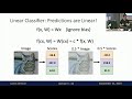
Understanding Linear Classifiers in Image Classification
Explore the role of linear classifiers in image classification and their effectiveness.

Introduction to Linear Predictors and Stochastic Gradient Descent
This lecture covers the fundamentals of linear predictors in machine learning, including feature extraction, weight vectors, and loss functions for classification and regression. It also explains optimization techniques like gradient descent and stochastic gradient descent, highlighting their practical implementation and differences.
Comprehensive Overview of Matrices and Determinants in Mathematics
In this session, Radhika Gandhi discusses the fundamental concepts of matrices and determinants, covering essential topics such as matrix properties, eigenvalues, eigenvectors, and various types of matrices. The session aims to provide a clear understanding of these concepts, which are crucial for mathematical problem-solving and exam preparation.
Most viewed summaries

A Comprehensive Guide to Using Stable Diffusion Forge UI
Explore the Stable Diffusion Forge UI, customizable settings, models, and more to enhance your image generation experience.

Kolonyalismo at Imperyalismo: Ang Kasaysayan ng Pagsakop sa Pilipinas
Tuklasin ang kasaysayan ng kolonyalismo at imperyalismo sa Pilipinas sa pamamagitan ni Ferdinand Magellan.

Mastering Inpainting with Stable Diffusion: Fix Mistakes and Enhance Your Images
Learn to fix mistakes and enhance images with Stable Diffusion's inpainting features effectively.

Pamamaraan at Patakarang Kolonyal ng mga Espanyol sa Pilipinas
Tuklasin ang mga pamamaraan at patakaran ng mga Espanyol sa Pilipinas, at ang epekto nito sa mga Pilipino.

How to Install and Configure Forge: A New Stable Diffusion Web UI
Learn to install and configure the new Forge web UI for Stable Diffusion, with tips on models and settings.

If you found this summary useful, consider buying us a coffee. It would help us a lot!