Introduction to Linear Predictors and Stochastic Gradient Descent

Okay. So let's, uh, get started with the actual, ah, technical content. So remember from last time,

we gave an overview of the class. We talked about different types of models that we're gonna explore: reflex models, state-based models, variable based models,

and logic models which we'll see throughout the course. But underlying all of this is, is, you know, machine learning. Because machine learning is what allows you to take data and, um,

tune the parameters of the model, so you don't have to, ah, work as hard designing the model. Um, so in this lecture,

I'm gonna start with the simplest of the models, the reflex based models, um, and show how machine learning can be applied to these type of models.

And throughout the class, ah, we're going to talk about different types of models and how learning will help with those as well.

So there's gonna be three parts, we're gonna talk about linear predictors, um, which includes classification regression, um,

loss minimization which is basically stating an objective function of how you, ah, want to train your machine learning model, and then stochastic gradient descent,

which is an algorithm that allows you to actually, ah, do the work. So let's start with, ah, perhaps the most,

um, cliched example of, uh, you know, machine learning. So you have- we wanted to do spam classification.

So the input is x, um, an email message. Um, and you wanna know whether an email message is spam or not spam.

Um, so we're gonna denote the output of the classifier to be Y which is in this case, either spam or not spam. And our goal is to, ah,

produce a predictor F, right? So a predictor in general is going to be a- a function that maps some input x to some output y.

In this case, it's gonna take an email message and map it to whether the email message is spam or not. Okay. So there- there's many types of prediction problems, um,

binary classification is the simplest one where the output is one of two, um, possibilities either yes or no. And we're gonna usually denote this as plus 1 or minus 1,

sometimes you'll also see 1 and 0. Um, there's regression where you're trying to predict a numerical value, for example, let's say housing price.

Um, there's a multi-class classification where Y is, ah, not just two items but possibly, um, 100 items, maybe cat, dog, truck,

tree, and different kind of image categories. Um, there's ranking where the output, um, is a permutation of the input, this can be useful.

For example, if the input is a set of, um, articles, or products, or webpages, and you want to rank them in some order to show to a user.

Um, structured prediction is where Y, ah, the output is an object that is much more complicated. Um, perhaps, it's a whole sentence or even an image.

And it's something that you have to kind of construct, you have to build this thing from scratch, it's not just a labeling.

Um, and there's many more types of prediction problems. Um, but underlying all of this, you know, whenever someone says I'm gonna do machine learning.

The first question you should ask is, okay what's the data? Because without data, there's no learning. So we're gonna call an example.

Um, x, y pair is something that specifies what the output should be when the input is x, okay? And a training data or a set of examples,

the training set is going to be simply a list or a multiset of, er, examples. So you can think about this as a partial specification of behavior. So remember, we're trying to design a system

that has certain- certain types of behaviors, and we're gonna show you examples of what that sum should do. If I have some email message that has CS221

then it's not spam but if it has, um, lots of, ah, dollar signs then there might, um, um, be spam.

Um, and, ah- so remember this is not a false specification behavior. These, ah, ten examples or even a million examples might not tell you what exactly this function is supposed to do.

It's just examples of, ah, what the function could do on those particular examples. Okay. So once you have this data,

so we're gonna use D_train to denote, ah, the data set. Remember, it's a set of input output pairs. Um, we're going to,

ah, push this into a learning algorithm or a learner. And what is the learning algorithm is gonna produce? It's gonna produce a predictor.

So predictors are F and the predictor remember is what? It's actually itself a function that, um, takes an input x and maps it to an output y.

Okay? So there's kind of two levels here. And you can understand this in terms of the, uh, modeling inferences of a learning paradigm.

So modeling is about the question of what should the types of predictors after you should consider are. Ah, inference is about how do you compute y given x?

And learning is about how you take data and produce a predictor so that you can do inference? Okay. Any questions about this so far?

[NOISE] So this is pretty high level and abstract and generic right now, and this is kinda, kind of on purpose because I wanna highlight how, um,

general machine learning is before going into the specifics of, uh, linear predictors, right? So this is an abstract framework.

Okay. So let's dig in a little bit to this actual, um, an actual problem. Um, so just to simplify,

ah, the email problem, let's, eh, consider the task of, um, predicting whether a string is an email address or not.

Okay. Um, so the input is an em-, ah, is a string and, ah, the output is- it's a binary classification problem,

it's either 1 if it's an email or minus 1 if it's not, that's what you want. Um, um, so the first step of, um, doing linear prediction is,

um, known as feature extraction. And the question you should ask yourself is, what properties of the input x might be relevant for predicting the output y?

Right, so I say, I really highlighted might be, right? At this point, you're not trying to encode the actual set of rules that solves a problem, that would involve no learning,

and that would just be trying to do it directly. But instead of- for learning you're kind of taking a, um, you know, a more of a backseat and you're saying,

"Well, here are some hints that could help you." Okay. Ah, so formally, a feature extractor takes an input and outputs a set of feature name,

feature value pairs, right? So I'll go through an example here. So if I have [email protected],

what are the properties that might be useful for determining whether a string is an email address or not? Well, you might consider the length of the string,

if it's greater than 10, maybe long strings are less likely to be email addresses than shorter ones. Um, and here, the feature name is length greater than 10.

So that's just kind of a label of that feature, and the value of that feature is 1, ah, representing it's true.

So it will be 0, if it's false. Here's another feature, the fraction of alphanumeric characters, right? So that happens to be 0.85 which is the number.

Um, there might be features that test for a particular, um, you know, letters for example, that it doesn't contain an "at" sign or that has a, you know,

feature value of 1 because there is an "at" sign, endsWith.com is one, endsWith.org is a 0 because that's not true. So, um, and there you could have many,

many more features, ah, and we'll talk more about features on next time. But the point is that you have a set of properties,

you're kind of distilling down this input which is could be a string, or could be an image, or could be something more complicated into kind of a um, you know, ground-up fashion that later,

we'll see how a machine learning algorithm can take advantage of. Okay. So you have this, ah, feature vector which has- is a list of

feature values and their associated names or labels. Okay. But later, we'll see that the- the names don't matter to the learning algorithm. So actually, what you should also think about

the feature vector is simply a list of numbers, and just kind of on the side make a note that all this, you know. position number three corresponds to contains "@" and so on.

Right, so I've distilled the- the email address [email protected] into the list of numbers 0- or 1, 0.85, 1, 1, 0.

Okay. So that's feature extraction. It's kind of distilling complex objects into lists of numbers which we'll see is what the kind of the lingua franca of these machine learning algorithms is.

Okay. So I'm gonna write some concepts on a board. There's gonna be a bunch of, um, concepts I'm going to introduce,

and I'll just keep them up on the board for reference. So feature vector is again an important notion and it's denoted Phi, um, of x on input.

So Phi itself- sometimes, you think about it, er, you call it the feature map which takes an input and returns, um, a vector, and this notation means that returns in general,

ah, d-dimensional vector, so a list of d numbers. And, um, the components of this feature vector we can write down as Phi_1, Phi_2, all the way to Phi_d of x.

Okay. So this notation is, eh, you know, convenient, um, because we're gonna start shifting our focus from thinking about

the features as properties of input to features as kind of mathematical objects. So in particular, Phi of x is a point in a high-dimensional space. So if you had two features,

that would be a point in two-dimensional space, but in general, you might have a million features, so that's a feature, ah,

it's a point enough, a hundred- ah, uh, million dimensional space. So, you know, it might be hard to think about that space, but well,

we'll see how we can, you know, deal with that in a later in a, in a bit. Okay. So- so that's a feature vector,

you take an input and return a list of numbers. Okay. Um, and now, the second piece is a weight vector.

So let me write down a weight vector. [NOISE] So a weight vector is going to be noted W.

Um, and this is also, uh, a list of D numbers. It's a point in a D-dimensional space

but we're gonna interpret it differently, as we'll see later. Okay. So- so a way to think about a weight vector is that, for each feature J.

So for example, frac of Alpha, um, we're gonna have a real number WJ, that represents the contribution of that feature to the prediction.

So this contribution is 0.6. So what does this 0.6 mean? So, so the way to think about this is that you have

your weight vector and you have a feature vector of a particular input, and you want- the score of, uh, your prediction is going to be, uh, the dot product between the weight vector and the feature vector.

Okay. So um, that's written W dot a phi of X um, which is um, written out as basically, looking at all the features and multiplying the feature of the value

times the weight of that feature and summing up all those numbers. So for this example, it will be minus 1.2,

that's the weight of the first feature, times 1, that's the feature value, plus 0.6 times 0.85 and so on.

And then, you get this number of 4.51 which is- happens to be the score for this example. Question?

So the feature extraction which is phi of X, is that, uh, supposed to be like an automated process or is it a part of manual extraction classification procedures?

Yeah. So the question is, is the feature extraction manual or automatic? So uh, phi is going to be implemented as a function like encode, right.

Um, you're going to write this function manually. But you know, the function itself is run automatically on examples. Um, later we'll see how you can actually learn features as well.

So you can slowly start to do less of a manual effort but uh, we're going to hold off until, next time for that.

Question? So we're talking about weight gaining and I know that in certain tests of regressions like,

uh, the weights being, uh, a percentage change, [inaudible] weights to percentage change of the outcome it doesn't, it doesn't mean the sphere?

Yeah. So the question is about interpretation of weights. Sometimes weights can have a more precise meaning. In general, um, you can,

you can try to read the tea leaves but it I don't think there is maybe, uh, in general a mathematically precise thing you can say about the meaning of individual weights.

But intuitively, and the intuition is important, is that you should think about each feature as you know, a little person that's going to make a vote on this prediction, right?

So you're voting either plus, yay or nay? And the weight of a particular feature is- specifies both the direction level whether- if positive weight means that,

um, that little person, um, is voting positive and negative weight means, that it's voting negative. The magnitude of that weight,

is how strongly that little person feels about the prediction, right? So, you know, contains add as three because maybe like "@" signs generally do occur in

email addresses but you know the fraction of alphanumeric characters, it's you know, less. So at that level,

you can have some intuition but the precise numbers and y is 0.6 versus 0.5. Um, that's, um, you can't really say much about that. Yeah. Another question? Does, uh, [inaudible] [NOISE] is it the same dot product for deeper networks.

They can feel like more weight vectors afterwards. It's still like it's, like just more than one products. [NOISE] So right now we're focusing on linear classifier.

So the question is what happens if you have a neural net with more layers? Um, there's gonna be more dot products but there's also goin- it's not just adding more features.

There's gonna be other uh, components which we'll get to in a later lecture. Yeah? Do the weights have to add up to a certain number or

how do you normalize it, so the weights, like you have to change the score value [inaudible] . Yeah. So the question is,

do the weights have to add up to something? Short answer is. No. There's obviously restricted settings, where you might want to normalize the weights or something but we're not gonna,

you know, uh, consider that right now. Later, we'll see that the magnitude of weight does tell you, you know, something. Okay, so, so just to summarize it's important to note that the weight vectors,

there's only one weight vector, right, you have to find one set of parameters for every- everybody. But the feature vector is per example.

So for every input, you get a new feature vector and the dot product of those two weighted combination of features is the uh, is the score. Okay, so, so now let's try to put the pieces together and define,

um, uh, of the actual predictor. All right, so remember we had this box with f in it, which takes x and returns y.

So what is inside that box? Um, and I'm hopefully giving you some intuition. Let me go to a board and write, uh, a few more things.

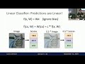
So the score, uh, remember is w dot phi of x. And this is just gonna be a number, um, and uh, the predictor.

So linear predictor actually let me call this linear. To be more precise, it's a linear classifier not just a predictor. Classifier is just a predictor that does classification.

Um, so a linear classifier um, denoted f of w. So f is where we're going to use, you know, predictors.

W just means that this predictor depends on a particular set of weights. And this predictor is, uh, going to look at the score and return the sign of that score.

So what is the sign? The sign looks at the score and says, is it a positive of a number? if it's positive then we're gonna return plus 1.

If it's a negative number, I'm gonna return minus 1. And if it's 0 then you know, I don't care. You can return plus 1 if you want, it doesn't matter.

Um, so what this is doing the remember the score is either, is a real number. So it's either gonna be kind of leaning towards um, you know, large value, large positive values or leaning towards,

uh, s- large small- negative values. And the sign basically says, okay you gotta commit are you- which side are you on? Are you on the positive side or you on the negative side?

And just kind of discretizes it. That's what the sign does. Okay.

Okay, so, so let's look at a simple example because I think a lot of what I've seen before is kind of more the, uh, formal machinery behind and the math behind how it works but it's

really useful to have some geometric intuition because then you can draw some pictures. Okay, so let's consider this, uh, case. So we have a weight vector which is 2, 1,

2 minus 1, and a feature vector which is a 2, 0, and another feature vector which is x0, 2 and 2, 4. Okay. So there's only two dimensions so I can try to draw them on a board.

So let's try to do that. Okay, so here is a two-dimensional plot. Um, and let's draw the fea- the weight vector first.

Okay so the weight vector is going to be at 2 minus 1. Okay. So that's this point. And the way to think about the weight vector is not the point.

Um, but actually um, the, the, the vector going from the origin to that point for reasons that will become clear later.

Okay so that's the, that's the weight. Okay. Um and then what about the other points so we have 2, 0, 0, 2. So 2, 0 is here,

0, 2 is here and 2, 4 is, uh, here. Right? Okay, so we have three points here. Okay, so, um, how do I think about what this weight vectors is, is doing?

So just for just for reference remember the classifier is looking at the sign of W dot, uh, phi of x. Okay. Um, so let's try to do uh, classification on these three points.

Okay so w is um, let me write it out formally, so 2, 1. Um, and this is 0, 2.

So what's the score when I do W dot phi of x here? It's 4, right? Because this is um, uh, 2, 0, 0, 2 um, 2, 4.

So this is just a dot product that's 4, um, and take the sign what's the sign of 4? One.

Okay. So that means I'm going to label this point as a positive, right? Positive point, okay what about 0, 2? Actually, sorry, this is just be a minus 1, right?

Okay. This is 2, minus 1. Okay, so if I take the dot product between this, I get minus 2 and then the sign of minus 2 is,

is minus 1, okay, so that's a minus. Um, and what about this one? So what's the dot product there? It's gonna be 0.

Okay. So, um, so this classifier will classify this point as a positive. This is a negative and this one I don't know. Okay. So we can fill in more points.

Um, but, but, you know, does anyone see kind of um, maybe a more general pattern? I don't wanna have to fill in the entire board with classifications.

Yeah? Orthogonal, everything to the right of it is positive and to the left of it is negative. Yeah so so let's try to draw the orthogonal.

Uh, this needs to go through that line. Okay, [NOISE] okay, so let's draw the orthogonal. So this is a right angle. Okay.

And, ah, what that gentleman said is that, the points- any point over here because it has acute angle width w, is going to be classified as positive.

So all of this stuff is um, you know, positive, positive, positive, positive, positive, and everything over here because it's an obtuse angle with w is going to be negative,

so everything over here is negative. And then, everything on this line is going to be 0. Okay? So, so I don't know.

Okay, and this line is called, um, the decision boundary, which is the concept not just for linear classifiers, but whenever you have any sort of classifier

the decision boundary is the separation between the regions of the space where the classification is positive versus negative. Okay? And in this case, um,

it's, it's separate because uh, we have linear classifiers, the decision boundary is straight, and we're just separating the, the space into two halves.

Um, if you were in three-dimensions, um, this vector would still be just a you know vector, but this decision, um,

boundary would be a plane. So you can think about it as you know coming out of the board if you want, but I'm not gonna try to draw that.

Um, and that's, that's kind of the geometric interpretation of how linear classifiers, ah, you know, work here. Question, yeah? It seems like your weight could be any values here.

Right? Yeah. So we have one last [inaudible].

Yeah. [inaudible] . Yeah. So that's a good point. So the, the observation is that,

no matter, if you scale this weight by 2, it's actually gonna still have the same decision boundaries. So the magnitude of the weight doesn't matter it's the direction that matters.

Um, so this is true for just making a prediction. Um, when we look at learning, ah, the magnitude of the weight will matter because we're going to,

you know, consider other more nuanced loss functions. Yeah. Okay. So let's move on. Any questions about linear predictors?

So, so, far what we've done is, we haven't done any learning. Right. If you've ah, you know, noticed,

we've just simply defined the set of predictors that we're interested in. So we have a feature vector, we have weight vectors, multiply them together, get a score and

then you can send them through a sign function and you get these linear classifiers. Right. There, there's no specification of data yet. Okay. So now, let's actually turn to do some learning.

So remember this framework, learning needs to take some data and return a predictor and our predictors are ah, specified by a weight vector.

So you can equivalently think about the learning algorithm as outputting a weight vector if you want for linear classifiers. Um, and let's unpack the learner.

So the learning algorithm is going to be based on optimization which we started ah, reviewing last lecture um, which separates ah, what you want to compute from how you want to compute it.

So we're going to first define an optimization problem which specifies what properties we want a- a classifier to have in terms of the data, and then we're going to figure out how to actually optimize this.

[NOISE] And this module is actually really really powerful um, and it allows people to go ahead and work on different types of criteria for and different types of models

separately from the people who actually develop general purpose algorithms. Um, and this has served kind of the field of machinery quite well. Okay. So let's start with an optimization problem.

So this is an important concept um, called a loss function and this is a super general idea that's using the machine learning and statistics.

So a loss function takes a particular example x, y and a weight vector, um, and returns a number and this number represents how unhappy we would be if we used the predictor

given by W to make a prediction on x when the correct output is y. Okay. So it's a little bit of a mouthful but, um, this basically is trying to characterize, you know,

if you handed me a classifier, and I go on to this example and try to classify it, is it gonna get it right or is it gonna get it wrong?

So high loss is bad ah, you don't wanna lose and low loss is good.

So normally, zero loss is the- the best you can then hope for. Okay. So let's do figure out the loss function for binary classification here. Um, so just some notation,

the correct label is, ah, denoted y and, um, the predicted label remember is um, the score, ah,

sent through the sign function and that's going to give you some particular label. Um, and let's look at this example. So w equals 2 minus 1 phi of x equals ah,

2, 0 and y equals minus 1. Okay. So we already defined the score as, um, one example is a w dot phi of x which is,

um, how co- confident we're predicting minu- plus 1. That's the way to, uh, you know, interpret this.

Okay. So um, what's the score of this, for this particular example again? It's 4.

Right. Um, which means I'm kind of, kinda positive that it's ah, you know, a plus 1. Yeah. Question?

Ah, I was wondering, is the loss function generally 1-dimensional or, or the output of the loss function? Yeah. So the- the question is whether the output of

loss function is usually a single number or not. Um, in most cases it is for basically all practical cases you should

think about the loss functions outputting a single number. The inputs can be, you know, a crazy high-dimensional. Yeah.

Why is it not 1-dimension? [NOISE] Um, there are cases where you might have multiple objectives that you're trying to optimize at once ah,

but in this class it's always gonna be, you know, 1-dimensional. Like maybe you care about, you know, both time and space or accuracy but robustness or something.

Sometimes you have multi-objective optimization. But that's way beyond the scope of this class. Okay. So we have a score.

Um, and now we're gonna define a margin. So let me, um. Okay. So let's, let's actually do this.

So we're talking about classification. I'm gonna sneak regression in a bit. So score is w dot phi of x.

This is how confident we are about plus 1, um, and the margin is the score ah, times y. Um, and this relies on y being plus 1 or minus 1.

So this might seem a little bit mysterious but let's try to, you know, decipher that, um here. Um, so in this example,

the score is 4. So what's the margin? You multiply by minus 1.

So the margin is, ah, minus 4. Right. And the margins interpretation is how correct we are. Right. So imagine the correct answer is ah,

if, if the score in the margin had the same sign, then you're gonna get positive numbers and then the, the confident, the more confident you are then the more correct you are.

Um, but if y is minus 1 and the score is positive, then the margin is gonna be negative which means that you're gonna be confidently wrong um, which is bad.

[LAUGHTER] Okay. So just to to see if we kind of understand what's going on. Um, so when is a binary classifier making a mistake on a given example.

Um, so I'm gonna ask for a kind of a show of hands. How many people think it's, it's when the margin is, uh, less than 0. Okay. I guess we can kind of stop there.

[LAUGHTER] I used to do these online quizzes where it was anonymous but we're not doing that this year.

Okay. So yes, the margin is less than 0. Um, when the margin is less than 0 that means y and the score are different signs which means that you're making a mistake.

[NOISE] Okay. So now we have the notion of a margin. Let's define ah, something called the

zero-one loss and it's called zero-one because it returns either a 0 or a 1. Okay. Very creative name. Um, so the loss function is simply,

did you make a mistake or not? Okay. So this notation let's try to decipher a bit. So if f of x here is the prediction when the input is x,

um, and not equal y is saying, did you make a mistake? So that's, think about it as a Boolean, and this one bracket is um, just notation.

It's called an indicator function that takes a condition and returns either a 1 or 0. So if ah, if the, the condition is true,

then it's gonna return a 1 and if the condition is false, it returns a 0. Okay. So all this is doing is basically returning a 1, if you made a mistake and 0,

if you didn't make a mistake. Okay. And we can write that as follows. We can write that as um,

the margin less or equal to 0. Right. Because pre- on the previous side of the margin is less than or equal to 0, then we've made a mistake and we should incur ah,

a loss of 1 and if the margin is greater than 0, then we didn't make a mistake and we should incur a loss of 0. Okay. All right so, um,

it will be useful to draw these loss functions, um, pictorially like this. Okay, so on the axi- x-axis here,

we're going to show the margin, right? Remember the margin is how, uh, correct you are. And on the, uh,

y-axis we're gonna show the- the loss function which is how much you're gonna suffer for it. Okay, so remember the margin,

if the margin is positive, that means you're getting it right which means that the loss is 0. But if the margin is less than 0,

that means you are getting it wrong and the loss is 1. Okay, so this is a 0-1 loss. That's, uh, thi- this thing- the visual that

you should have in mind when you think about zero-one loss. Yeah. [NOISE] Like less than 0 because we are not defining the event actually 0 [inaudible] classified as correct.

Yeah, so there is this kind of boundary condition of when ex- what happens exactly at 0 that I'm trying to sweep under the rug because it's not, um, terribly important. Um, here, it's less we go to 0 to be kind of on the safe side.

So if you don't know you're also, uh, gonna get it wrong. Um, otherwise you could always

just return 0 and then you, that, you don't want that. Okay. So is it- uh, any questions about, uh,

kind of binary classification so far. So we've set up these linear predictors and I've defined the 0-1 loss as a way to capture, um,

how unhappy we would be if we had a classifier that was, ah, operating on a particular data point x, y. So, um, just to-

I'm gonna go on a little bit of a digression and talk about linear regression. Um, uh, um, [NOISE] and, and the reason I'm doing this is that

loss minimization is such a powerful and general framework, and it go- transcends, you know, all of these, you know,

linear classifiers, regression, setups. So I want to kind of emphasize over- the overall story. So I'm gonna give you a bunch of different examples, um, classification,

linear regression side-by-side so we can actually see how they compare and hopefully, their- the common denominator will kind of emerge more, um, clearly from that. Okay, so we talked a little bit about linear regression in the last lecture, right?

So linear regression in some sense is simpler than classification because if you have a linear, uh, uh, predictor, um,

and you get the score w dot phi of x, it's already a real number. So in linear regression,

you simply return that real number and you call that your prediction. Okay? Okay so now we- let's move towards defining our loss function. Um, so there's gonna be, uh,

a concept that's gonna be useful, it's called the residual, um, which is, as- against kind of trying to capture how,

uh, wrong you are. Um, so here is a particular linear, uh, predictor, um, linear regresser, um, and it's making predictions all along,

you know, for different values of x. Um, and here's a data point of Phi of xy. Okay? So the residual is the difference between,

um, the true value y and the predictor value y. Okay, um, and in particular it's the amount by which, um, the prediction is overshooting the, you know, target.

Okay, so this is- this is a difference. Um, and if you square the [NOISE] difference you get something called, uh, the squared loss.

[NOISE] So this is something we mentioned last lecture. Um, residual can be either negative or [NOISE] positive.

Um, but errors, either, if you're very positive or very negative, that's bad and squaring them makes it so that you're gonna, you know,

suffer equally for, um, errors in both, you know, directions. Okay, so the square loss is the residual squared.

So let's do this kind of simple example. So here we have our weight vector 2 minus 1. The feature vector is 2, 0. What's the score?

It's 4, y is minus 1. So, uh, the residual is 4 minus minus 1 which is 5 and, uh, 5 squared is 25.

So the squared loss on this particular example is 25. Okay, so let's plot this. So just like we did it for a 0-1 loss.

Let's see what this loss function looks like. So the, the horizontal axis here instead of being the margin is going to be this quantity,

uh, for regression called the residual. Um, it's going to be the difference between the prediction and the, the true target. And I'm gonna plot the loss function.

Um, and this loss function is just, you know, the squared function, right? So with- if the residual is 0,

then the loss is 0. If as a residual grows in either direction, then I'm going to pay,

uh, something for it. And it's a quadratic penalty which means that, um, it actually grows,

you know, uh, pretty fast. So if I'm, you know, the residual is 10 then I'm paying 100.

Okay, so, so that's the squared loss. Um, there's also another loss. I'll throw in here,

um, called the absolute deviation loss. And this might actually be the last thought, if you didn't know about regression you might, uh, immediately come to.

It's basically the absolute difference between the prediction and, um, the, the actual true target. [NOISE] Um, turns out the squared loss.

The- there's a kind of a longer discussion about, you know, which loss function, um, you know, makes sense.

The- the salient points here are that the absolute deviation loss is kind it has this kink here. Um, and so it's not smooth.

Sometimes it makes it harder to optimize, um, but the squared loss also has this kind of thing that blows up, which means that it's, uh, uh,

it really doesn't like having outliers or, uh, really large values because it's gonna, you- you're gonna pay a lot for it.

Um, but at this level, just think about this as, you know, different losses. There's also something called a Huber loss which kind of, uh, um,

combines both of these, is smooth, and also grows linearly instead of quadratically. Um, okay, so we have both classification and regression.

We can define margins and residuals. We get either, uh, different loss functions out of it.

Right? Um, and now we want to minimize the loss. Okay? Um, so it turns out that for one example and this is really easy, right? So if I- if I told you,

okay, how do I minimize the loss here? Well, okay, it's 0. Done. [NOISE] So that- that's not super interesting. And this corresponds to the fact that,

you know, if you have a classifier, you're just trying to fit one point, um, it's really not that hard. So that's kind of not the point.

[NOISE] The point of machine learning is that you have to fit all of them. Remember, you only get one weight vector, you have all of these examples,

you have a million examples. And you want to find one weight vector that kind of balances, uh, errors across all of them.

And in general, you might not be able to achieve loss of 0, right? So tough luck . Life is hard. Ah, so you have to make trade-offs, you know,

which examples are you going to kind of sacrifice for the good of other examples. And this is kind of actually a lot of where, you know, issues around fairness of machine learning actually come in

because in cases where you can't actually make a prediction that's, you know, equally good for everyone. You know, how do you actually, you know,

responsibly make these trade-offs. Um, but, you know, that's a- that's a broader topic.

Let's just focus on trade-off defined by the simple sum over all the loss examples. So lets just say we want to minimize the average loss over all the examples. Okay, so once we have these loss functions,

if you average [NOISE] over the training set, you get something which we're gonna call a train loss. Um, and that's a function of W. Right?

So loss is on a particular example. Train loss is on the entire data set. [NOISE]

Okay. So any questions about this, uh, so far? Okay. So there is this, uh, discussion about which regression loss to use, which I'm gonna skip.

Um, you can feel free to read it in the notes if you're interested. The punchline is that if you want things that look like the mean square loss, if you want things that look like the median,

use the absolute deviation loss. Um, but I'll skip that for now. Yeah? [inaudible] regression like this.

Uh, when do people start thinking of regressions like in terms of loss minimization? Yeah. Uh, so regression has,

Least Squares Regression is from like the early 1800s. Um, so it's been around for is- you know, kind of, you can call it the first machine learning that was ever done,

um, if you- if you want, um, I guess the loss minimization framework is, um, it's hard to kind of pinpoint a particular point in time, you know,

it's kind of not a terribly, uh, um, er, er, you know, it's not like, uh, um, you know,

innovation in some sense. It's just more of a- at least right now it's kind of a pedagogical tool to organize, um, all the different methods that exist. Yeah.

Say I'm training on mean and median. Do you mean that like, uh, in that particular training, training set, the median would be the [NOISE] highest accuracy and the most confident,

whereas like with, uh, loss [inaudible] deviation would be the median instead of the mean? Yeah. So, um, I don't wanna get into these examples but, uh, bri- briefly,

if you have three points that you- you can't exactly f- fit perfectly, um, you- if you use absolute deviation, then you're gonna find the median value.

You're gonna basically predict the median value. And if you use the square loss, you're gonna predict the mean value.

But, um, I'm happy to talk offline [NOISE] if- if you want. [NOISE] Okay. So what we've talked about so far is we have

these wonderful linear predictors which are driven by feature vectors and weight vectors, and now we can define a bunch of different loss functions that capture, you know, how we care about,

um, you know, regression and classification. And now let's try to actually do some real, uh, machine learning. How, how do you actually optimize these objectives?

So remember the learner is going, uh, so now we've talked about the optimization problem which is minimizing the training loss. Um, we'll come back to that next lecture.

Um, and then now we're gonna talk about optimization algorithm. Okay? So what is a optimization problem? Now, remember last time we said, okay,

let's just abstract away from the details a little bit. Let's not worry about if it's, uh, the square loss or s- you know,

some other loss. [NOISE] Um, let's just think about as a kind of abstract function. So one-dimension, the training loss might look something like this.

You have a single weight and for each weight you have a number which is your loss on your training samples. [NOISE] Okay? And you want to find this point.

So in two dimensions, um, it looks something like this. Yeah. Let me try and actually draw this because I think it'll,

[NOISE] uh, be, um, useful in a bit to solve, let me pull this up. [NOISE] Okay. So in two dimensions,

um, what optimization looks like is as follows. So I'm gonna- I'm now plotting, um, W_1 and W_2 which are the two components of this two-dimensional weight vector.

For every point I have a weight vector and that value is gonna be the loss, the training loss. Um, and it's, er, you know,

[NOISE] it's pretty standard in these settings to draw what are called level curves. Um, so let's do this. So each curve here is a ring of points where,

uh, the function value is identical. So if you, uh, look at terrain maps, those are level curves. So you know, kind of what I'm talking about.

So this is the minimum and as you kind of grow out you get larger and larger, um. Okay. I'll keep on doing this for a little bit. Okay. [NOISE] All right.

Um. [NOISE] And, uh, the goal is to find the minimum. Okay. All right. So how are we gonna do this?

So yeah, question. Assuming that there is a single minimum. Yeah, why am I assuming,

uh, there is a single minimum. [NOISE] in general for arbitrary loss functions, there is not necessary a single minimum,

I'm just doing this for simplicity. It turns out to be true for, um, you know, uh, many of these linear classifiers.

[NOISE] Okay. So last time we talked about gradient descent, right? And the idea behind gradient descent is that well, I don't know where this is.

So let's just start at 0, [NOISE] as good as any place. And what I'm gonna do at 0 is I'm gonna compute the gradient.

So the gradient is this vector that's, uh, perpendicular to the level curves. So the gradient is gonna point in this direction.

That says, hey, in this direction is where the function is increasing the most dramatically. Um, and gradient descent says,

um, takes- goes in the opposite direction, right? Because remember we wanna minimize loss. Um, so I'm gonna go here.

And, um, now I'll hopefully reduce my, uh, function value, not necessarily but, um, we hope that's- that's the case.

Now, we compute, uh, the gradient [NOISE] again. The gradient says, um, you know, maybe it's pointing this way.

So I go in that direction and maybe now it's, uh, pointing this way. And I keep on going.

Um, this is a little bit made up. Um, but hopefully, eventually I get to the, um, the [NOISE] origin.

And you know, I'm, I'm kind of simplifying things quite a bit here. So in- there's a whole field of optimization that studies exactly what kind of functions you can optimize and how gradient descent when it works and when it doesn't.

Um, I'm just gonna kind of go through the mechanics now and defer the kind of the formal proofs of when this actually works until, um, later. Okay. So that's kind of the- the schema of how gradient descent works.

So in code this looks like this. So initialize at 0 and then loop in some number of iterations, um, which let's- for simplicity just think there's a fixed number of iterations.

And then, I'm gonna pick up my weights, compute the gradient, move in the opposite direction, and then there's gonna be a step size that, uh,

tells me how fast I want to, you know, make progress. Okay? And we'll come back to,

you know, uh, what, uh, the step size, uh, does later. Okay. So let's specialize it to a least squares, uh, regression.

So we kind of did this last week, but, um, just to kind of review, um. So the training loss for least squares regression is this.

So remember it's an average over the loss of individual examples, and the loss of a particular example is the residual squared. So that's this expression.

Um, and then all we have to do is compute the gradient. And you know, if you remember your calculus, it's just I've used the chain rule.

So this two comes down here. You have the, um, you know, the residual times the derivative of what's inside

here and the gradient with respect to W is, uh, phi of x. Okay. So last time we did this in Python in 1-dimension. So 1-dimension, and hopefully all of you should feel comfortable doing

this because this is just kind of basic, um, calculus. Um, here we have w is a vector. So, uh, we're not taking derivatives but we're taking gradients.

Um, so there's, you know, some things to be, uh, wary of but in this case it's often kind of useful to double-check that.

Well, um, the gradient version actually matches, uh, the, the single-dimensional version as well because last time remember we have the x out here.

Um, and one thing to note here is that, um, there's a prediction minus target, and that's the residual. So the gradient is driven by,

um, you know, kind of this quantity. So if the prediction equals the target, uh, what's the gradient? It's going to be 0 which is kind of what you want.

If you're already getting the answer correct, then you shouldn't want to move your, uh, your weights, right? So often you know we can do things in the abstract and everything will work.

But you know it's, it's often a good idea to write down some objective functions, take the gradient and see if gradient descent on using these gradients that you computed is kind of a sensible thing because there's

kind of many layers you can understand and get intuition for this stuff at the kind of abstract level optimization or kind of at the algorithmic level. Like you pick up an example is it sensible to update when

the gradient other than when the prediction equals the target. Okay, so so let's take the code that we have from our, from last time, and I'm going to expand on it a little bit,

and hopefully set the stage for doing stochastic gradient. Um, okay. So, so last time we had gradient descent.

Okay, so remember last time we defined a set of points, we defined the function which is the train loss here. Um, we defined the derivative of the function, and then we have gradient descent.

Okay, um, so I'm gonna do a little bit of housecleaning and I'm just, uh, um, don't mind me. Um, okay so I'm gonna make this a little bit more explicit,

what this algorithm is. Gradient descent depends on, um, a function, a derivative of a function and let say, um, you know,

the dimensionality, um, and I can call this gradient FDF and in this case it's, uh, D where D equals 2. Okay, and I want to kind of separate.

This is the kind of algorithms and this is, you know, modeling. So this is what we want to compute and this is, you know, how we compute it. [NOISE]

Okay and this code should still work. Okay, um. All right, so what I'm gonna do now is, um, upgrade this to vector.

So remember the x here is just a number, right? But we want to support vectors. Um, so in Python,

um, we're going to import NumPy so which is this, uh, nice vector and matrix library um, and, um, I'm gonna make some,

you know, arrays here, um, which this is just going to be a one-dimensional array. So it's not that exciting.

So this, this w dot x becomes, uh, the actual dot I need to call. And I think w needs to be np.zeros(d).

Okay. All right. So that's just- should still run actually, sorry, this is 1-dimensional.

Okay. So remember last time we ran this, uh, this program and, um, it starts out with some weights and then it

converges to 0.8 and the function value kind of keeps on going on. Okay. All right, so let's, let's try to, um,

you know it's really hard to kind of see you whether this algorithm is any, doing anything interesting because we only have two points, it's kind of trivial.

So how do we go about, um, you know, because I'm going to also implement stochastic gradient descent. How do we have kind of a test case to see if this algorithm is, you know, working?

Um, so there's kind of this technique which I, I really like [NOISE] which is to call, generate artificial data and ideas that, you know, what is learning.

You're learning as you're taking a dataset and you're trying to fit- find the, the weights that best fit our dataset. Uh, but in general if I generate some arbitrary,

if I downloaded a dataset I have no idea what the right kind of quote unquote right answer is. So there's a technique where I go backwards and say,

okay let's let's decide what the right answer is. So let's say the right answer is, um, 1, 2, 3, 4, 5.

So it's a 5-dimensional problem. Okay. Um, and I'm going to generate some data based on that so that this, uh, weight vector is kind of good for that data.

Um, I'm going to skip all my breaks in this lecture. Um, so I'm going to generate a bunch of points. So let's generate 10,000 point.

The nice thing about artificial data is you can generate as much as you'd want. Um, there's a question, yeah? A true w?

So true w just means like the, the correct, the ground truth, the w. The true y, true output or?

So w is a weight vector. So this is kind of going backwards. Remember, I want to fit the weight vector

but um, I'm just kind of saying this is the right answer. So I want to make sure that the algorithm actually recovers this later. Okay, so I'm going to generate some random data.

So there's a nice function, random.randn which generates a random d-dimensional vector and y. I'm gonna set- what should I set y to?

Which side of w you want? Yeah. So I'm gonna do regressions. So I want to do, uh,

true_w dot uh, x, right? So I mean if you think about it, if I took this data and I

found the, the like true one- w is the right thing that we'll get 0 loss here. Okay. But I'm going to make your life a little bit

more interesting and we're gonna add some noise. Okay, so let's print out what that looks like. Also I should add it to my dataset.

So okay, so this is my dataset. Okay, I mean, I can't really tell what's going on but, but you can look at the code and you, you can assure yourself that,

uh, this data has structure in it. [NOISE] Okay, so let's get rid of this print statement and let's train and see what happens. So let's.

Okay. Oh, one thing I forgot to do. Um, so if you notice that the objective functions that I've, uh, written down they haven't divided by the number of data points.

I want the average loss, not the, the sum. Um, it turns out that, you know if you have the sum, then things get really big and you know, blow up.

So let me just normalize that. Okay. So let me lock it. Okay, so it's training, it's training.

Um, actually so let me, uh, do more iterations. So I did 100 iterations, let's do 1000 iterations.

Okay. So when the function value is going down, that's always something to- you know, good to check. Um, and you can see the weights are kind of slowly getting to,

you know, what appears to be 1, 2, 3, 4, 5, right? Okay. So this is a hard proof but it's kind of

evidence that this learning algorithm is actually kind of doing the right thing. Um, okay so now let's see if I add, you know more points.

So I now have 100,000 points. Now, you know, obviously it gets slower, um, and you'll, you know, hopefully get there you know,

one day but I'm just gonna kill it. Okay, any questions about, uh, oops, my terminal got screwed up.

Okay. So what did I do here, I defined loss functions, took their derivatives. Um, the gradient descent is what we implemented last time and the only thing different

I did, this time is generated data sets so I can kind of check whether gradient descent is working. Yeah question. So the fact that the gradient is just the residual [inaudible]

a algorithm to learn from overpredictions versus like underpredictions? The question is whether the fact that the gradient is residual allows the algorithm to learn from under or over predictions.

Um, yeah. So the gradient is if you think about it, yeah that's good intuition. So if you look at, um,

if you're over-predicting, right? That means the gradient is kind of- assume that this is like 1. So that means this is going to be positive which means that, hey if you opt that way,

you're going to over-predict more and more and incur more loss. So, um, by subtracting a gradient, you're kind of pushing the weights out in

the other direction and same for when you're, um, you're under-predicting. Yeah, so that's good intuition to have. Yeah.

What is the effect of the noise when you generate [inaudible] What is the effect of the noise? Um, the effect of the noise,

it makes the problem a little bit, you know, harder so that it takes more examples to learn. Um, if you shut off the noise then it will- you know, we can try that.

Um, I've never done this before, but presumably you'll learn, you know, f- faster, but maybe not.

Um, the noise isn't, you know, that much. But, um, okay. So, so let's say you have,

you know, like 500 examp- 1000 examples. You know, that's quite a few examples. As in now, you know, this algorithm runs,

you know, pretty slowly, right? And in- in modern machine learning you have, you know, millions or hundreds of millions of examples.

So gradient descent is gonna be, you know, pretty slow. So how can we speed things up a little bit, and what's the problem here?

Well, if you look at the- the- what the algorithm is doing, it's iterating. And each iteration it's computing the gradient of the training loss. And the training loss is,

um, average of all the points, which means that you have to go through all the points and you compute the lo- gradient of the loss and you add everything up.

And that's what is expensive and, you know, it takes time. So, you know, you might wonder, well, how, how can you avoid this?

I mean, you- if you wanted to do gradient descent you have to go through all your points. Um, and the, the key insight behind stochastic gradient descent is that, well maybe- maybe you don't have to do that.

So, um, maybe- you know, here- here's some intuition, right? So what is- what is this gradient?

So this gradient is actually the sum of all the gradients from all the examples in your training set. Right? So we have 500,000 points adding to that.

So actually what this gradient is- is, um, it's actually kind of a sum of different things which are maybe pointing in slightly different directions which all average out to this direction.

Okay. So maybe you can actually not average all of them, but you can, um, average just a couple or maybe even in an

extreme case you can just like take one of them and just, you know, march in that direction. So, so here's the idea behind stochastic gradient descent.

So instead of doing gradient descent, we are going to change the algorithm to say for each example in the training set, I'm just going to pick it up and just update, you know.

It's- instead of like sitting down and looking at all of the training examples and thinking really hard, I'm just gonna pick up one training example and update right away.

So again, the key idea here is, it's not about quality it's about, uh, quantity. May be not the world's best life lesson,

but it seems to work in- it works in here. Um, and then, there's also this question of what should the step size be? And in- generally, in stochastic gradient descent,

it's actually even a bit more important because, um, when you're updating on each- each individual example, you're getting kind of noisy estimates of the actual gradient.

And, uh, and people often ask me like, "Oh, how should I set my step size and all." And the answer is like there is no formula.

I mean, there are formulas, but there's no kind of definitive answer. Here's some general guidance.

Um, so if step size is small, so really close to 0, that means you are taking tiny steps, right?

That means that it'll take longer to get where you want to go, but you're kind of proceeding cautiously. so it's less likely you're gonna,

you know- uh, if you mess up and go in the wrong direction you're not gonna go too far in the wrong direction. Um, conversely, if you have it to be really,

really, large then, you know, it's like a race car. You, kind of, drive really fast, but you might just kind of bounce around a lot.

So, pictorially what this looks like is that, you know, here's maybe a moderate step size, but if you're taking steps,

really big steps, um, you might go over here and then you jump around and then maybe, maybe you'll end up in the right place but maybe

sometimes you can actually get flung off out of orbit and diverge to infinity which is a bad situation. Um, so there's many ways to set the step size.

You can set it to a, you know, constant. You can- usually, you have to, um, you know, tune it.

Or you can set it to be decreasing the intuition being that as you optimize and get closer to the optimum, you kind of want to slow down, right?

Like if you- you're coming on the freeway, you're driving really fast, but once you get to your house you probably don't want to be like driving 60 miles an hour.

Okay. So- actually I didn't implement stochastic gradient. So let me do that. So let's, let's try to get stochastic gradient up and going here. Okay. So, so the interface to stochastic gradient changes.

So- right? So the- in gradients then all you need is a function. And it just kind of computes the sum over all the training examples. Um, so in stochastic gradient,

I'm just going to denote S as for stochastic gradient. I'm gonna take an index I, and I'm going to update on the Ith point only.

So I'm going to only compute the loss on the Ith point. And same for its derivative. Um, you can look at the Ith point,

um, and just compute the gradient on that Ith point. Okay? And this should be called SDF. Okay. So now instead of doing gradient descent,

let's do stochastic gradient descent. And I'm going to pass in sf, sdf, d, and, um, the number of points because I need to know how many points there are now.

Um, copy gradient descent, and it's basically kind of the same function. I'm just going to stick another for loop there.

So stochastic gradient descent, it's going to take the stochastic functions, stochastic gradient, the dimensionality and- Okay?

So now, before I was just going through, um, number of iterations and now, right, I'm not going to try to compute the value of the- all the training examples.

I'm going to, um, loop over all the points and I'm going to call just evaluate the function at that point I,

and compute the gradient at that point I instead of the entire, you know, dataset. And then everything else is the same. I mean, one other thing I'll do here is that I'll use a different step size schedule.

So um, 1 divided by number of updates. So I want it so that the number of, uh, the step size is gonna decrease over time.

Okay, so I start with a equals 1 and then it's half, and then it's a third, and it's a fourth, and it keeps on going down. Um, sometimes you can put a square root and that's more typical in some cases,

but, um, I'm not going to worry about the details too much. Uh, question? The point I is the chosen randomly but here we just [inaudible]. Yes. The question is- the word

stochastic means that there should be some randomness here. And, you know, technically speaking, the- the stochastic gradient descent is where

you're sampling a random point and then you're updating on it. I'm cheating a little bit, um, uh, because I'm iterating over all the points.

You know, in practice if you have a lot of points and you randomize the order it's kind of- it's- it's similar but it's- there is a kind of a technical difference that I'm trying to hide.

Okay. So- so this is stochastic gradient descent. Um, to iterate, you know, go over all the points and just, you know update.

Okay? Um, so let's see if this works. Um, okay. I don't think that worked.

[LAUGHTER] Maybe- let's see what happened here? I did try it on 100,000 points. Maybe that works.

And, nope, doesn't work either. Um, anyone see the problem? [inaudible]

So I'm printing this, um, out, uh, at the- at the end, um, of each iteration.

So that should be fine, um. Really, this should work. So gradient descent was working, right?

Maybe I'll, I'll try- It's probably not the best idea to be debugging this live. Okay. Let's, let's make sure gradient descent works.

Um, okay, so that was working right. Okay. So stochastic gradient descent. I mean, it's really fast and converges,

[LAUGHTER] but it doesn't converge to the right answer. I think [inaudible].

Yeah, but that should get incremented to 1. So that- It might be true.

Okay, so I do have a version of this code that does work. [LAUGHTER] So what am I doing here, that's different.

Okay, I'll have some water. Maybe I need some water. [LAUGHTER] Okay, so this version works. Yeah.

[inaudible] Yeah, that's- that's probably good. That's a good call. Yeah. okay.

All right. Now, it works. Thank you. [LAUGHTER] Um, so yeah.

Yeah, this is a good lesson. Um, it's that when you're dividing, um, these needs to be one- actually in Python 3,

this is not a problem but I'm so- on Python 2 for some reason. But this should be, uh, 1.0 divided by numUpdates. Otherwise, I was getting-

So how is it faster? Okay. So why is it faster? [LAUGHTER].

Yeah, okay. Okay. Let's- let's, uh, go back to 500,000, okay.

Okay. So one full sweep over the data is the same amount of time. But you notice that immediately, it already converges to 1, 2,

3, 4, 5, right? So this is like way, way faster than gradient descent. Remember, I just, uh, kind of compare it.

Um, gradient descent is, um, you run it. And after one stop, it's, like,

not even close. Right. Yeah? What noise levels you have to have until gradient descent becomes better?

What noise levels you have to have until gradient descent becomes better? Um, so it is true that if you have more noise, then gradient descent might be, uh,

stochastic gradient descent can be unstable. Um, there might be ways to mitigate that with step size choices. But, um, yeah, probably,

you have to add a lot of noise for stochastic gradient to be, um, really bad. Um, I mean, this is in some sense, you know, if you take a step back and think about what's going on in this problem,

it's a 5-dimensional problem. There's only five numbers and I'm feeding it half a million data points, right? There, there aren't- there's not that much to learn here.

And so there's a lot of redundancy in the dataset. And generally, actually, this is true. I go into a large dataset,

there's gonna be a lot of, you know, redundancy. So, uh, going through all of the data and then try to make an informed decision is, you know, pretty wasteful, where sometimes you can

just kind of get a representative sample from, um, one example or more as common to do the like of kind of mini-batches where you maybe grab a hundred examples

and you update on that which is- so there's a way to be somewhere in between stochastic gradient and gradient descent. Okay, let me move on. Um.

Okay. Summary so far, we have linear predictors, um, which are based on scores.

So linear predictors we include both classifiers and regressors, um, we can do loss minimization, and we can, uh,

if we implement it correctly, we can do, uh, SGD. Okay. So that was- I'm kind of switching things.

I hope you are kind of following along. I'll introduced binary classification and then, I did all the optimization for linear regression.

So now, let's go back to classification and see if we could do stochastic gradient descent here. Okay. So for classification, remember,

we decided that the zero-one loss is the thing we want. We want to minimize the number of mistakes. You know, who can argue with that?

Um, so rem- remember, what is zero-one loss look like? It looks like this. Okay? So what happens if I try to run stochastic gradient descent on this? Um, I mean, I can run the code,

but [OVERLAPPING] yeah, it's- it won't work, right? And why won't it work? [inaudible].

Yeah. So two popular answers are it's not differentiable, that's- it's one problem. Um, but I think that the- the bigger problem and kind of deeper problem is that,

what is the- what is the gradient? Zero. Zero. It's like zero, basically everywhere except for this point,

which are, you know, it doesn't really matter. So, um, so as- as we learned that if you try to update with a gradient of 0, um, then you, you won't move your weights, right?

So gradient descent will not work on the zero-one, uh, loss. Um, so that's- that's kind of unfortunate. So how should we fix this problem? Yeah?

[inaudible] Yeah, let's, let's make the gradient non-zero. Let's skew things. Um, so there's one loss,

which I'm gonna introduce called the hinge loss, which, uh, does exactly that. Um, so let me write the hinge loss down.

And the hinge loss, um, is basically, uh, is zero here when the margin is greater than or equal to 1 and rises linearly.

So if you've gotten it correct by a margin of 1 so you're kind of pretty safely on the err side of, um, getting it correct, then we won't charge you anything.

But as soon as you start, you know, dip into this area, we're gonna charge you a kind of a linear amount and your loss is gonna grow linearly.

Um, so there's some reasons why this is a good idea. So it upper bounds the zero-one loss, um, it's, uh, it has a property called- known as convexity,

which means that if you actually run the gradient descent, you're actually gonna converge to the global optimum. Um, I'm not gonna get into that.

And so that's, you know, that's a hinge loss. Um, so what remains to be done is to compute the gradient of this,

you know, hinge loss, okay? So how do you compute this gradient? So in some sense, it's a trick question because

the gradient doesn't exist because it's not, um, you know, differentiable everywhere, but we're gonna pre- pretend that little point doesn't exist, okay?

So, so what is this hinge loss? The hinge loss is actually two functions, right? There is a zero function here and then there's like this,

uh, 1 minus x function. So what am I plotting here? I'm plotting the- the margin and, uh, the loss.

Okay? So this is, uh, the zero function, and this is, uh,

1 minus, uh, w dot phi of xy. And the hinge loss is just the maxima of these two functions. So at every point,

I'm just taking the top function. So um, that's how I am able to trace out, uh, this- this curve.

Okay? All right. So if I want to take the gradient of this function, you know, you, you can try to do the math.

Well, let's think through it. You know, what- what should the gradient be? Um, we're, we're here,

what should the gradient be? It's zero. And if I'm here, what should the gradient be? It should be the- whatever the gradient of this function is, right?

So in general, when you have a gradient of this- of this kind of max, uh, you have to kind of break it up into cases. Um, and depending on where you are,

um, you, you have a different case. So loss is equal to- if I'm over here, and what's the condition for being over here?

If the margin is greater than 1, right? And then otherwise, I'm going to take the gradient of this with respect to w, which is gonna be minus phi of x y, you know, otherwise.

Okay? Um, so again, we can try to interpret the, the gradient of the hinge loss. So remember your stochastic gradient descent, you have a weight vector,

and you're gonna pick up an example and you say, Oh, let's compute the gradient move away from it. So if you're getting the example right,

then the gradient zero don't move, which is the right thing to do. And otherwise, you're going to move in that direction because you're minus, minus of phi of x y,

which kind of imprints this example into your weight vector. So- and you can formally show that it actually increases your, uh, margin after you do this.

Okay? Yeah? What's the significance of the margin being 1? What's the significance of the margin being 1?

Um, this is a little bit arbitrary, you're just kind of sending a non-zero value. Um, and, and, you know,

in support vector machines, you set it to 1, and then you have regularization on the weights and that gives you, uh, some interpretation.

So I don't have time to go over that right now, but, uh, feel free to ask me later. There's another loss function.

Uh, do you have a question? Yeah. Why is the or why do we choose the margin if it's a loss function that's supposed on the square or another loop?

Yeah. So why do you choose the margin? So in classification, we're gonna look at the margin because that tells you how comfortable when you're predicting,

uh, co- you know, correctly. In regression, you're gonna look at residuals and square losses. So it depends on what kind of- what problem you're trying to solve.

Um, just really quickly, some of you might have heard of logistic regression. Logistic regression is this, uh,

yellow loss function, right? So the point of this is saying that this loss minimization framework is, you know, really general and a lot of things that you might have heard of

least squares logistic regression are a kind of a special case of this. So if you kind of master how to do loss minimization, you kind of, uh, can do it all.

Okay. So summary, um, basically, what's on the board here? If you're doing classification,

you take the score which comes from the, uh, w dot phi of x and you drive it into the sign, and then you get either plus 1 or minus 1.

Regression, you just use a score. Now to train, you have to assess how well you're doing. In classification, there's a notion of a margin.

Res- uh, in regression, it's the residual, and then you can define loss functions. And here is we only talking about five loss functions but there's many others, um,

especially for a kind of structure prediction or ranking problems, there's all sorts of different loss functions. But they're kind of based on these simple ideas of,

you know, you have a hinge, the upper balance is zero-one if you're doing classification and, [NOISE] um, some sort of square-like error for, you know, regression.

And then, once you have your loss function, provided it's not zero-one, you can optimize it using, um, SGD, which turns out to be a lot faster than, you know, gradient descent.

Okay. So next time, we're gonna talk about, uh, Phi of x, which we've kind of left as, you know, someone just hands it to you.

And then we're also gonna talk about what is the really true objective of machine learning? Is it really to optimize the training loss?

Okay, until next time.