Introduction to Residues in Complex Analysis
Residues play a crucial role in evaluating complex integrals via the Understanding the Residue Theorem in Complex Variables. This summary explores three key techniques to calculate the residue of a complex function at a given pole.
Technique 1: Using Laurent Series Expansion
- Concept: Residue at a point (z_0) is the coefficient (b_1) of the ((z - z_0)^{-1}) term in the Laurent series expansion of the function around (z_0).
- Application: Expand the function into its Laurent series and identify the (b_1) coefficient directly.
- Example: For (f(z) = \frac{\sin z}{z^2}) at (z=0):
- (\sin z) Taylor expansion: (z - \frac{z^3}{3!} + \frac{z^5}{5!} - \ldots)
- Dividing by (z^2), we get: [ \frac{\sin z}{z^2} = \frac{1}{z} - \frac{z}{3!} + \frac{z^3}{5!} - \ldots ]
- Residue (coefficient of (1/z)) is 1.
This technique relies on understanding the Understanding Laurent Series and Residues in Complex Analysis to effectively identify the coefficient.
Technique 2: Limit Method for Simple Poles
- Definition: A simple pole at (z_0) means the Laurent series principal part has only the (b_1 / (z - z_0)) term.
- Method: Calculate the residue as: [ \text{Res}{z = z_0} f(z) = \lim{z \to z_0} (z - z_0) f(z) ]
- Proof Idea: Multiplying by (z - z_0) cancels the singularity; other analytic terms vanish at the limit, isolating the residue.
- Pole Check:
- Limit zero: no pole at (z_0)
- Finite nonzero limit: simple pole
- Infinite limit: higher order pole
- Example: Find residue of (\frac{\cos z}{z^4 - 1}) at (z = i):
- Factor denominator: (z^4 - 1 = (z - i)(z + i)(z^2 - 1))
- Residue: [ \lim_{z \to i} (z - i) \frac{\cos z}{(z - i)(z + i)(z^2 - 1)} = \frac{\cos i}{(i + i)(i^2 - 1)} ]
- Using Euler’s formula to compute (\cos i = \frac{e + e^{-1}}{2}), residue equals (\frac{e + e^{-1}}{8 i}).
This method complements the understanding provided in Introduction to Functions of Complex Variables and Holomorphicity regarding singularities and their classification.
Technique 3: General Formula for Higher Order Poles
- Setup: For a pole of order (n) at (z_0), choose an integer (m \geq n).
- Steps:
- Multiply (f(z)) by ((z - z_0)^m)
- Differentiate this product (m - 1) times: [ \frac{d^{m-1}}{dz^{m-1}} \left[(z - z_0)^m f(z)\right] ]
- Evaluate at (z = z_0) and divide by ((m - 1)!)
- Result: This equals the residue of (f(z)) at (z_0).
- Proof Sketch: Differentiation reduces powers and isolates (b_1), the residue coefficient.
- Example: Compute residue of (\frac{z \cos z}{(z - \pi)^3}) at (z = \pi):
- Multiply by ((z - \pi)^3) to get (z \cos z)
- Differentiate twice (since (m = 3), (m - 1 = 2)): [ \frac{d^2}{dz^2} (z \cos z) = -2 \sin z - z \cos z ]
- Evaluate at (z = \pi): (-2 \sin \pi - \pi \cos \pi = 0 + \pi = \pi)
- Divide by (2! = 2) to get residue (\frac{\pi}{2}).
Differentiation and dealing with holomorphic functions and their derivatives relate to concepts in Understanding Cauchy-Riemann Relations and Holomorphic Functions.
Summary
| Technique | Pole Type | Formula | Usage | |----------------------------|--------------------|-----------------------------------------------------|-----------------------------------------------| | Laurent Series Coefficient | Any pole | Extract (b_1) from series | When Laurent expansion is available | | Limit Method | Simple pole | (\lim_{z \to z_0} (z - z_0) f(z)) | Quick residue calculation, pole identification | | Differentiation Method | Higher order poles | (\frac{1}{(m - 1)!} \left[\frac{d^{m-1}}{dz^{m-1}} ((z - z_0)^m f(z)) \right]_{z=z_0}) | Residues at higher order poles |
Understanding these techniques equips you with powerful tools to evaluate complex integrals, analyze pole behavior, and apply the Understanding the Residue Theorem in Complex Variables effectively.
Greetings students and welcome back to another video on complex variables. In this lesson, I'm going to state and
prove three well-known techniques that allow you to find the residues of a complex function. This is going to come
in handy when applying the residue theorem and when integrating complicated real functions as we'll see in the next
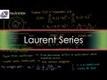
video. So, let's start. Suppose I have a complex function with the following la. Recall from my Laurance series video
that a Luron series is essentially a generalized tailaylor series that includes rational expressions which have
negative powers on Z. In other words, the B series or the principal part in addition to the polomial portion that
you find in a typical tailaylor series or the analytical part, this a series. Recall also that the residue of a
function f of z at a particular point z knot is the coefficient b1 in the lauron expansion of f of z around z knot. So
this B1 right here, the coefficient of the 1 / Z minus Z knot term. This very brief explanation actually gives rise to
the first technique used to find the residue of f of Z at Z knot, which just involves finding the Lauron expansion of
f of Z around Z knot and then just taking out the B1 from that lauron expansion. I don't really need to prove
this considering that this is after all the definition of the residue. So let's just skip straight to an example. In
this example, we want to find the residue of sin z / z ^2 at z= 0. This is fairly simple. We know that the
tailaylor expansion or the power series representation for sin z about z= 0 is given by z - z cub over 3 factorial plus
z 5 factorial and so on. That means the luron expansion of sin z / z ^ 2 would just be this tailaylor expansion of sin
z / z ^ 2. And if we simplify everything then we'll get 1 / z minus z over 3 factorial plus z cubed over 5 factorial
and so on and the powers will keep getting higher as we keep going. So the residue of sin z over z ^2 at 0 is just
the coefficient of the 1 / z minus 0 or 1 / z term which in this case is just one.
The second technique I'm going to talk about doesn't involve finding the lauron expansion. It applies to cases where you
can't find the Lauron expansion or you just don't want to. It specifically applies to when your function f of z has
a simple pole at z knot and you want to find the residue at that simple pole. Recall that by a simple pole I mean a
pole about which the lauron expansion of f of z only goes up to the 1 / z minus z kn term in the lauron expansion. In
other words, this summation in the principal part up here only has b1 as the non-trivial term. Everything else is
just zero. The second technique is also pretty simple. All you do is multiply the function f of z by z minus z knot
and take the limit as z approaches z knot. Proving this technique is also fairly simple. So let's suppose for the
proof that f of z has a lauron expansion about z knot given by the following expression. You know the one we
mentioned above. Now because z knot is a simple pole of f of z. This b series here only goes up till j = 1. So the
laur expansion of f of z can be simplified to the following. The sum from k= 0 to infinity of a k * z - z k
plus b1 / z - z kn. So now the principal part contains just the b1 term. Let's now multiply both sides by z minus
z kn to get the following equation. Now what happens when we take the limit of both sides as Z approaches Z knot? Well,
this first summation term goes away since it contains powers of Z minus Z KN greater than or equal to 1. On the other
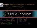
hand, the second term, the constant B1, the residue, it just stays there. So we can say that the residue of a complex
function f of z at a simple pole z is just the limit as z approaches z knot of zus z kn * f of z. Now just to clarify
the reason we use the limit is that f of z is actually undefined at z knot. Z knot is still a pole after all even
though it's a simple pole and if you multiply f of z by z minus z knot and evaluate the whole result at z knot you
would just end up with the 0 / 0 which is undetermined. So that's why we've used the limit. So you technically don't
get 0 / 0 and everything turns out okay. Let's now do an example to illustrate this technique. In this example, we want
to find the residue of cossine z / z 4 - 1 at z = i. Let's begin by factoring the denominator. So when we multiply by z -
z kn, which in this case is zus i, then we can more easily cancel out the terms. You know that z 4 - 1 is just z ^ 2 - 1
* z ^2 + 1 and that z ^2 + 1 is just z - i * z + i. So let's just plug this factored form into the equation for f of
z and this is what we'll get. Now because cossine z is continuous and differentiable or holorphic at z= i.
That means z= i must be a simple pole since z minus i only appears once in the denominator.
So that means we can use technique number two to find the residue at z= i because z= i is a simple pole and
technique number two only applies to finding residues at simple poles. In this case, the residue is just the
limit as Z approaches I of Z - I * cosine Z / Z ^ 2 - 1 * Z - I Z + I. And if we cancel the Z minus I terms, we end
up with this equation. Now, if we want to take the limit of this expression at Z= I, we can do that very easily just by
substituting in Z= I. The denominator becomes -2 * 2 I, which is -4 I. But the tricky bit is with the numerator. And
even if you try to use a calculator that has complex numbers, you end up with a math error. Still, there's a trick you
can use to evaluate cosine I using the oiler formula. And with the oiler formula, you can isolate and find an
expression for cosine z in terms of just exponentials. I leave it up to the viewer to show that cossine z is e i z +
e i z / 2. It's kind of like cossine x which is e to x + e x / 2. You might be able to see the analogy there. If you
use this equation for cosine z, then you'll find that cossine i is just e + e inverse / 2. So the residue of cosine z
over z 4 - 1 at z= i is just e + e inverse over 8 i. And that solves our example. Now, before using technique
number two, you might wonder, how do I know if the function has a simple pole at Z= Z KN? What if it's a pole of
higher order? Or what if it doesn't even have poles? How can I find that out before using technique number two? Well,
the answer lies in the Lauron series* ZUS Z KN expression I wrote up here, which I'll copy paste below. Now if I
didn't have a pole at Z knot, then all my B coefficients would be zero since my function would be completely analytic at
that point. Therefore, if I then took the limit of this expression as Z approaches Z KN, then I would just end
up with a zero residue. However, if my Z knot was a higher order pole, then in addition to the B1 term in
my B series, I would also have a B2 term and even terms beyond B2 up to the order of the pole. Of course, note that the
terms beyond B2 have one less power on the Z minus Z knot in the denominator, mainly because we've already multiplied
it out once. Now if I take the limit of this expression as Z approaches Z knot then
because of these extra terms corresponding to the higher order pole we get infinity for the limit. Therefore
if I then took the limit of Z minus Z knot * f of z when z knot is a higher order pole I get infinity. So that's how
you can tell you have a simple pole. If this limit is zero then the function doesn't have a pole at z knot and it's
totally analytic there. When this limit is infinity, the pole at Z knot is a higher order pole. And when the limit is
a nonzero finite number, then you do have a simple pole at Znot. And the limit is just the residue B1. So this
quantity, this limit isn't just a way to calculate residues for simple poles. It's also a diagnostic tool to check
whether or not you even have a simple pole at Znot. And that completes the discussion for
technique number two. Let's go to the third and final residue calculation technique. And the second technique you
saw just applied to simple pole zen knot. This technique number three is an extension and it now applies to higher
order poles. It's not as easy as the other ones. And let me begin first by describing how it works.
Suppose you want to find the residue of the function f of z at z= z knot. And z knot turns out to be a non-simple pole.
Turns out to be a higher order pole. In fact, suppose that the order of the pole z is n. So what you do is you start by
multiplying f of z by z minus z kn to the power m where m is some integer that's greater than or equal to the
order of the pole n. Then what you do is you differentiate zus z to the m * f of z m minus1 times and the third step is
to divide that derivative by m -1 factorial and then evaluate the result at the pole z knot and then this final
quantity is your residue at the nons simple pole z knot. Now when it comes to proving this technique the book I was
reading just said that the proof was very simple and left it as an exercise to the reader. I'm not like that. Well,
sometimes. So, following the famous words of the tank commander/ headcoach legend Byron Scott, I'm going to man up
and prove this technique to you. Let's start with the lauron series of f of z. Now, when znot is a pole of order n, we
can expand out the b series so that it goes until the b subn term. Now, let's start with the first step of
technique three. multiply f of z by z minus z kn the power m where m is an integer greater than or equal to n. Now
because m is greater than or equal to n all these powers of z minus z knot in the principal series the b series all
those powers are going to be positive which makes differentiation more straightforward. Now let's apply the
second step and differentiate this whole expression m minus1 times. If we do that then all the powers on the z minus z kn
terms in this a series will reduce by m minus one and we'll also be multiplying the coefficient a subk by k + m * k + m
-1 * all the way to k + 2. This is just using the chain rule and applying it to the differentiation of polomials.
But what about the principal part? Well, if you differentiate the principal part mus1 times, then every term which has a
power less than mus1 will become zero. That's because if you differentiate a polomial, the degrees or powers on that
polomial are going to keep decreasing with every differentiation until you get a constant term and when you
differentiate that constant term, you get zero. Therefore, all the terms in the B series except for B1 become zero.
The B1 term on the other hand is going to have its power reduced by the number of times we differentiate. So, m minus
one. In addition, because the power comes down as a coefficient every time we differentiate, we'll also have mus1
factorial multiplying b1. And now it's time for the final step of the technique where we evaluate the derivative at z= z
knot and divide by mus1 factorial. If we evaluate the derivative at z= z knot, every term in this a series is going to
be zero, leaving only the b1 term. and dividing that by m minus one factorial will just give us the residue b1 at z= z
knot. So that's it. We've proven the validity of technique number three that if you have a higher order pole at z
knot, you can multiply that function with that higher order pole whose residue you want to find by z minus z
kned to the power of an integer m greater than or equal to the order of the pole. Then you can differentiate
that m minus one times and then divide by m minus one factorial and evaluate the derivative at that higher order pole
z knot to get the residue. Let's finish off the video with one last example applying this third technique.
In this example, we want to find the residue of z cosine z / zus p<unk> cubed at z= pi. We can already see from the
function that the numerator z cosine z doesn't have any poles at z= pi which means that the denominator is the only
factor contributing to the z= pi pole and since the denominator contains zus p<unk> cubed we can conclude that z=
p<unk> is a third order pole. So let's use technique number three and multiply f of z by zus p<unk> cubed leaving us
with only z cosine z. Now because we multiplied by Z -<unk> cubed, we have to differentiate this expression 3 -1
times. In other words, we find the second derivative. You can use the product rule to show that the second
derivative here is just -2 sin zus z cosine z. Finally, in the third step, we'll substitute z=<unk> and divide by
the factorial of 3 - 1, which is just 2. Sin pi is zero while cosine pi is 1. So for the residue, we'll end up with
p<unk> by 2. And that should do it for the video. If you enjoyed the lecture, feel free to like and subscribe. In the
next complex variables video, we'll talk about how to use the residue theorem to determine integrals, a video that some
of you have already requested. Thank you for watching and this is the faculty of Khan signing out.
Yes. For (f(z) = \frac{\cos z}{z^4 - 1}) at (z = i), factor the denominator as ((z - i)(z + i)(z^2 - 1)). The residue is (\lim_{z \to i} (z - i) f(z) = \frac{\cos i}{(i + i)(i^2 - 1)}). Using Euler's formula, (\cos i = \frac{e + e^{-1}}{2}), the residue simplifies to (\frac{e + e^{-1}}{8i}).
A residue is the coefficient of the (1/(z - z_0)) term in the Laurent series expansion of a complex function around a pole (z_0). It is important because residues allow us to evaluate complex integrals efficiently, especially through the Residue Theorem, which simplifies calculating contour integrals by summing residues at poles inside the contour.
To calculate the residue via Laurent series, expand the function around the pole (z_0) into its Laurent series and identify the coefficient (b_1) of the ((z - z_0)^{-1}) term. This coefficient is the residue. For example, for (f(z) = \frac{\sin z}{z^2}) at (z = 0), expanding (\sin z) as (z - z^3/3! + ...) and dividing by (z^2) shows the (1/z) term has coefficient 1, so the residue is 1.
The limit method calculates the residue at a simple pole (z_0) by evaluating (\lim_{z \to z_0} (z - z_0) f(z)). This limit isolates the coefficient of the singular term. If the limit is finite and nonzero, the point is a simple pole and the limit equals the residue. If zero or infinite, it indicates no pole or higher-order pole, respectively.
For a pole of order (n) at (z_0), multiply the function by ((z - z_0)^m) with (m \geq n), differentiate the product (m - 1) times, evaluate at (z = z_0), then divide by ((m-1)!). This gives the residue. For example, for (f(z) = \frac{z \cos z}{(z - \pi)^3}), multiply by ((z - \pi)^3) to get (z \cos z), differentiate twice, evaluate at (z=\pi), and divide by 2! to find the residue (\frac{\pi}{2}).
When using the limit method (\lim_{z \to z_0} (z - z_0) f(z)), if the limit equals zero, there is no pole at (z_0); if it is a finite nonzero value, (z_0) is a simple pole; if the limit is infinite, the pole is of higher order. This helps classify the singularity before applying the appropriate residue calculation technique.
Use the Laurent series method when the function’s series expansion around the pole is readily available or easy to compute, as it directly identifies the residue coefficient. The differentiation method is more suited for higher order poles where the series expansion is complicated; it uses derivatives to systematically isolate the residue without full expansion.
Heads up!
This summary and transcript were automatically generated using AI with the Free YouTube Transcript Summary Tool by LunaNotes.
Generate a summary for freeRelated Summaries
Understanding Laurent Series and Residues in Complex Analysis
This lecture explains Laurent series as a powerful generalization of Taylor series used to expand complex functions, especially around singularities. It covers how Laurent expansions include both analytic and principal parts, defines singularities such as poles and essential singularities, and introduces the residue concept fundamental to the residue theorem.
Understanding the Residue Theorem in Complex Variables
This guide explains the residue theorem, a fundamental concept in complex variables, detailing how contour integrals around singular points relate to residues. It includes a step-by-step proof leveraging Laurant series expansions and Cauchy's theorem, providing clarity on why residues determine integral values.
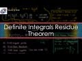
Using the Residue Theorem to Evaluate Definite Integrals Involving Sine and Cosine
This video lesson demonstrates how to apply the residue theorem from complex analysis to evaluate definite integrals involving sine and cosine functions. It explains transforming trigonometric integrals into contour integrals on the unit circle using complex exponentials, then finding residues at singularities to compute the integrals efficiently, including examples with detailed calculations.
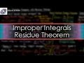
Using the Residue Theorem to Evaluate Improper Integrals
This lecture explains how to apply the residue theorem from complex analysis to compute improper integrals over infinite intervals, including a detailed example involving rational functions and the Cauchy principal value. Key takeaways include conditions for convergence, the role of even functions, and a step-by-step residue calculation method.

Computing Improper Fourier Integrals Using Complex Analysis Techniques
Learn how to evaluate improper integrals involving sine and cosine from negative to positive infinity using complex contour integration, residue theorem, and Jordan's lemma. This guide explains replacing trigonometric terms with complex exponentials, identifying poles, and applying these theorems to compute Fourier integrals with detailed example solutions.
Most Viewed Summaries

A Comprehensive Guide to Using Stable Diffusion Forge UI
Explore the Stable Diffusion Forge UI, customizable settings, models, and more to enhance your image generation experience.

Kolonyalismo at Imperyalismo: Ang Kasaysayan ng Pagsakop sa Pilipinas
Tuklasin ang kasaysayan ng kolonyalismo at imperyalismo sa Pilipinas sa pamamagitan ni Ferdinand Magellan.

Mastering Inpainting with Stable Diffusion: Fix Mistakes and Enhance Your Images
Learn to fix mistakes and enhance images with Stable Diffusion's inpainting features effectively.

Pamamaraan at Patakarang Kolonyal ng mga Espanyol sa Pilipinas
Tuklasin ang mga pamamaraan at patakaran ng mga Espanyol sa Pilipinas, at ang epekto nito sa mga Pilipino.

How to Install and Configure Forge: A New Stable Diffusion Web UI
Learn to install and configure the new Forge web UI for Stable Diffusion, with tips on models and settings.

If you found this summary useful, consider buying us a coffee. It would help us a lot!