Understanding Entropy: The Connection Between States and Thermodynamics

If you followed some of the mathematics, and some of the thermodynamic principles in the last several videos, what occurs in this video might just blow your mind.

So not to set expectations too high, let's just start off with it. So let's say I have a container.

And in that container, I have gas particles. Inside of that container, they're bouncing around like gas particles tend to do, creating some pressure on the

container of a certain volume. And let's say I have n particles. Now, each of these particles could be

in x different states. Let me write that down. What do I mean by state?

Well, let's say I take particle A. Let me make particle A a different color. Particle A could be down here in this corner, and it could

have some velocity like that. It could also be in that corner and have a velocity like that.

Those would be two different states. It could be up here, and have a velocity like that. It could be there and have a velocity like that.

If you were to add up all the different states, and there would be a gazillion, of them, you would get x. That blue particle could have x different states.

You don't know. We're just saying, look. I have this container.

It's got n particles. So we just know that each of them could be in x different states.

Now, if each of them can be in x different states, how many total configurations are there for the system as a whole? Well, particle A could be in x different states, and then

particle B could be in x different places. So times x. If we just had two particles, then you would multiply all

the different places where X could be times all the different places where the red particle could be, then you'd get all the different configurations for the system.

But we don't have just two particles. We have n particles. So for every particle, you'd multiply it times the number

of states it could have, and you do that a total of n times. And this is really just combinatorics here.

You do it n times. This system would have n configurations. For example, if I had two particles, each particle had

three different potential states, how many different configurations could there be? Well, for every three that one particle could have, the other

one could have three different states, so you'd have nine different states. You'd multiply them.

If you had another particle with three different states, you'd multiply that by three, so you have 27 different states.

Here we have n particles. Each of them could be in x different states. So the total number of configurations we have for our

system-- x times itself n times is just x to the n. So we have x to the n states in our system. Now, let's say that we like thinking about how many states

a system can have. Certain states have less-- for example, if I had fewer particles, I would have fewer potential states.

Or maybe if I had a smaller container, I would also have fewer potential states. There would be fewer potential places for our little

particles to exist. So I want to create some type of state variable that tells me, well, how many states can my system be in?

So this is kind of a macrostate variable. It tells me, how many states can my system be in? And let's call it s for states.

For the first time in thermodynamics, we're actually using a letter that in some way is related to what we're actually trying to measure.

s for states. And since the states, they can grow really large, let's say I like to take the logarithm of the number of states.

Now this is just how I'm defining my state variable. I get to define it. So I get to put a logarithm out front.

So let me just put a logarithm. So in this case, it would be the logarithm of my number of states-- so it would be x to the n, where this is number of

potential states. And you know, we need some kind of scaling factor. Maybe I'll change the units eventually.

So let me put a little constant out front. Every good formula needs a constant to get our units right.

I'll make that a lowercase k. So that's my definition. I call this my state variable.

If you give me a system, I should, in theory, be able to tell you how many states the system can take on. Fair enough.

So let me close that box right there. Now let's say that I were to take my box that I had-- let me copy and paste it.

I take that box. And it just so happens that there was an adjacent box next to it.

They share this wall. They're identical in size, although what I just drew isn't identical in size.

But they're close enough. They're identical in size. And what I do, is I blow away this wall.

I just evaporate it, all of a sudden. It just disappears. So this wall just disappears.

Now, what's going to happen? Well, as soon as I blow away this wall, this is very much not an isostatic process.

Right? All hell's going to break loose. I'm going to blow away this wall, and you know, the

particles that were about to bounce off the wall are just going to keep going. Right?

They're going to keep going until they can maybe bounce off of that wall. So right when I blow away this wall, there's no pressure

here, because these guys have nothing to bounce off to. While these guys don't know anything. They don't know anything until they come over here and say,

oh, no wall. So the pressure is in flux. Even the volume is in flux, as these guys make their way

across the entire expanse of the new volume. So everything is in flux. Right?

And so what's our new volume? If we call this volume, what's this? This is now 2 times the volume.

Let's think about some of the other state variables we know. We know that the pressure is going to go down. We can even relate it, because we know that our

volume is twice it. Is 2 times the volume. What about the temperature?

Well, the temperature change. Temperature is average kinetic energy, right? Or it's a measure of average kinetic energy.

So all of these molecules here, each of them have kinetic energy. They could be different amounts of kinetic energy, but

temperature is a measure of average kinetic energy. Now, if I blow away this wall, does that change the kinetic energy of these molecules?

No! It doesn't change it at all. So the temperature is constant.

So if this is T1, then the temperature of this system here is T1. And you might say, hey, Sal, wait, that doesn't make sense.

In the past, when my cylinder expanded, my temperature went down. And the reason why the temperature went down in that

case is because your molecules were doing work. They expanded the container itself. They pushed up the cylinder.

So they expended some of their kinetic energy to do the work. In this case, I just blew away that wall. These guys did no work whatsoever, so they didn't

have to expend any of their kinetic energy to do any work. So their temperature did not change. So that's interesting.

Fair enough. Well, in this new world, what happens? Eventually I get to a situation where my molecules

fill the container. Right? We know that from common sense.

And if you think about it on a microlevel, why does that happen? It's not a mystery.

You know, on this direction, things were bouncing and they keep bouncing. But when they go here, there used to be a wall, and then

they'll just keep going, and then they'll start bouncing here. So when you have gazillion particles doing a gazillion of

these bounces, eventually, they're just as likely to be here as they are over there. Now.

Let's do our computation again. In our old situation, when we just looked at this, each particle could be in one of x places, or in one of x states.

Now it could be in twice as many states, right? Now, each particle could be in 2x different states. Why do I say 2x?

Because I have twice the area to be in. Now, the states aren't just, you know, position in space. But everything else-- so, you know, before here, maybe I had

a positions in space times b positions, or b momentums, you know, where those are all the different momentums, and that was equal to x.

Now I have 2a positions in volume that I could be in. I have twice the volume to deal with. So I have 2a positions in volume I can be at, but my

momentum states are going to still be-- I just have b momentum states-- so this is equal to 2x. I now can be in 2x different states, just because I have 2

times the volume to travel around in, right? So how many states are there for the system? Well, each particle can be in 2x states.

So this is 2x times 2x times 2x. And I'm going to do that n times. So my new s-- so this is, you know, let's call this s

initial-- so my s final, my new way of measuring my states, is going to be equal to that little constant that I threw in there, times the natural log of the

new number of states. So what is it? It's 2x to the n power.

So my question to you is, what is my change in s when I blew away the wall? You know, there was this room here the entire time, although

these particles really didn't care because this wall was there. So what is the change in s when I blew away this wall?

And this should be clear. The temperature didn't change, because no kinetic energy was expended.

And this is all in isolation. I should have said. It's adiabatic.

There's no transfer of heat. So that's also why the temperature didn't change. So what is our change in s?

Our change in s is equal to our s final minus our s initial, which is equal to-- what's our s final? It's this expression, right here.

It is k times the natural log--and we can write this as 2 to the n, x to the n. That's just exponent rules.

And from that, we're going to subtract out our initial s value, which was this. k natural log of x to the n. Now we can use our logarithm properties to say, well, you

know, you take the logarithm of a minus the logarithm of b, you can just divide them. So this is equal to k-- you could factor that out-- times

the logarithm of 2 to the N-- it's uppercase N, so let me do that. This is uppercase N.

I don't want to get confused with Moles. Uppercase N is the number of particles we actually have. So it's 2 to upper case N times x to the uppercase N divided by

x to the uppercase N. So these two cancel out. So our change in s is equal to k times the natural log of 2

to the N-- or, if we wanted to use our logarithm properties, we could throw that N out front. And we could say, our change in the s, whatever this state

variable I've defined-- and this is a different definition than I did in the last video-- is equal to big N, the number of molecules we have, times my little constant, times the

natural log of 2. So by blowing away that wall and giving my molecules twice as much volume to travel around in, my change in this

little state function I defined is Nk the natural log of 2. And what really happened?

I mean, it clearly went up, right? I clearly have a positive value here. Natural log of 2 is a positive value.

N is positive value. It's going to be very large number than the number of molecules we had.

And I'm assuming my constant I threw on there is a positive value. But what am I really describing?

I'm saying that look, by blowing away that wall, my system can take on more states. There's more different things it can do.

And I'll throw a little word out here. Its entropy has gone up. Well, actually, let's just define s

to be the word entropy. We'll talk more about the word in the future. Its entropy has gone up, which means the number of states we

have has gone up. I shouldn't use the word entropy without just saying, entropy I'm defining as equal to S.

But let's just keep it with s. s for states. The number of states we're dealing with has gone up, and it's gone up by this factor.

Actually, it's gone up by a factor of 2 to the n. And that's why it becomes n natural log of 2. Fair enough.

Now you're saying, OK. This is nice, Sal. You have this statistical way, or I guess you could, this

combinatoric way of measuring how many states this system can take on. And you looked at the actual molecules.

You weren't looking at the kind of macrostates. And you were able to do that. You came up with this macrostate that says, that's

essentially saying, how many states can I have? But how does that relate to that s that defined in the previous video?

Remember, in the previous video, I was looking for state function that dealt with heat. And I defined s, or change in s-- I defined as change in s--

to be equal to the heat added to the system divided by the temperature that the heat was added at. So let's see if we can see whether these things are

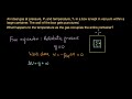
somehow related. So let's go back to our system, and go to a PV diagram, and see if we can do anything useful with that.

Alright. OK. So this is pressure, this is volume.

Now. When we started off, before we blew away the wall, we had some pressure and some volume.

So this is V1. And then we blew away the wall, and we got to-- Actually, let me do it a little bit differently.

I want that to be just right there. Let me make it right there. So that is our V1.

This is our original state that we're in. So state initial, or however we want it. That's our initial pressure.

And then we blew away the wall, and our volume doubled, right? So we could call this 2V1.

Our volume doubled, our pressure would have gone down, and we're here. Right?

That's our state 2. That's this scenario right here, after we blew away the wall.

Now, what we did was not a quasistatic process. I can't draw the path here, because right when I blew away the wall, all hell broke loose, and things like

pressure and volume weren't well defined. Eventually it got back to an equilibrium where this filled the container, and nothing else was in flux.

And we could go back to here, and we could say, OK, now the pressure and the volume is this. But we don't know what happened in between that.

So if we wanted to figure out our Q/T, or the heat into the system, we learned in the last video, the heat added to the system is equal to the work done by the system.

We'd be at a loss, because the work done by the system is the area under some curve, but there's no curve to speak of here, because our system wasn't defined while all the

hell had broke loose. So what can we do? Well, remember, this is a state function.

And this is a state function. And I showed that in the last video. So it shouldn't be dependent on how we got

from there to there. Right? So this change in entropy-- actually, let me be careful

with my words. This change in s, so s2 minus s1, should be independent of the process that got me from s1 to s2.

So this is independent of whatever crazy path-- I mean, I could have taken some crazy, quasistatic path like that, right?

So any path that goes from this s1 to this s2 will have the same heat going into the system, or should have the same-- let me take that--

Any system that goes from s1 to s2, regardless of its path, will have the same change in entropy, or their same change in s.

Because their s was something here, and it's something different over here. And you just take the difference between the two.

So what's a system that we know that can do that? Well, let's say that we did an isothermal. And we know that these are all the same isotherm, right?

We know that the temperature didn't change. I told you that. Because no kinetic energy was expended, and none of the

particles did any work. So we can say, we can think of a theoretical process in which instead of doing something like that, we could have had a

situation where we started off with our original container with our molecules in it. We could have put a reservoir here that's equivalent to the

temperature that we're at. And then this could have been a piston that was maybe, we were pushing on it with some rocks that are pushing in the

left-wards direction. And we slowly and slowly remove the rocks, so that these gases could push the piston and do some work, and

fill this entire volume, or twice the volume. And then the temperature would have been kept constant by this heat reservoir.

So this type of a process is kind of a sideways version of what I've done in the Carnot diagrams. That would be described like this.

You'd go from this state to that state, and it would be a quasistatic static process along an isotherm. So it would look like that.

So you could have a curve there. Now, for that process, what is the area under the curve there?

Well, the area under the curve is just the integral-- and we've done this multiple times-- from our initial volume to our second volume, which is twice it, of p times

our change in volume, right? p is our height, times our little changes in volume, give us each rectangle.

And then the integral is just the sum along all of these. So that's essentially the work that this system does. Right?

And the work that this system does, since we are on an isotherm, it is equal to the heat added to the system. Because our internal energy didn't change.

So what is this? We've done this multiple times, but I'll redo it. So this is equal to the integral of V1 to 2V1.

PV equals NRT, right? NRT. So P is equal to NRT/V.

NRT over V dv. And the t is T1. Now, all of this is happening along an isotherm, so all of

these terms are constant. So this is equal to the integral from V1 to 2V1 of NRT1 times 1 over V dv.

I've done this integral multiple times. And so this is equal to-- I'll skip a couple of steps here, because I've done it in several videos already-- the

natural log of 2V1 over V1, right? The antiderivative of this is the natural log. Take the natural log of that minus the natural log of that,

which is equal to the natural log of 2V1 over V1. Which is just the same thing as NRT1 times the natural log of 2.

Interesting. Now, let's add one little one little interesting thing to this to this equation.

So this is NRT, but if I wanted to write in terms of the number of molecules, N is the number of moles. So I could rewrite N as the number of molecules we have

divided by, 6 times 10 to the 23 power. Right? That's what n could be written as.

So if we do it that way, then what is our-- remember, all of this, we were trying to find the amount of work done by our system.

Right? But if we do it this way, this equation will turn into-- so let's see.

The work done by our system-- this is our quasistatic processes that's going from this state to that state, but it's doing it in a quasistatic way, so that we can get an

area under the curve. So the work done by this system is equal to-- I'll just write it.

N times R over 6 times 10 to the 23, times T1 natural log of 2. Fair enough.

Let's make this into some new constant. For convenience, let me call it a lowercase k. So the work we did is equal to the number of particles we

had, times some new constant-- we'll call that Boltzmann constant, so it's really just 8 divided by that. Times T1, times the natural log of 2.

Fair enough. Now, that's only in this situation. The other situation did no work, right?

So I can't talk about this system doing any work. But this system did do some work. And since it did it along an isotherm, delta-- the change

in internal energy is equal to 0, so the change in internal energy, which is equal to the heat applied to the system minus the work done by the system-- this is going to be

equal to 0, since our temperature didn't change. So the work is going to be equal to the heat added to the system.

So the heat added to the system by our little reservoir there is going to be-- so the heat is going to be the number of particles we had times Boltzmann constant, times our

temperature that we're on the isotherm, times the natural log of 2. And all this is a byproduct of the fact that

we doubled our volume. Now, in the last video, I defined change in s as equal to Q divided by the heat added, divided by the

temperature at which I'm adding it. So for this system, this quasistatic system, what was the change in s?

How much did our s-term, our s-state, change by? So change in s is equal to heat added divided by our temperature.

Our temperature is T1, so that's equal to this thing. Nk T1 times the natural log of 2, all of that over T1. So our delta-- these cancel out.

And our change in our s-quantity is equal to Nk times the natural log of 2. Now, you should be starting to experience an a-ha moment.

When we defined in the previous video, we were just playing with thermodynamics, and we said, gee, we'd really like to have a state variable that deals with heat, and we

just made up this thing right here that said, change in that state variable is equal to the heat applied to the system divided by the temperature at which the heat was applied.

And when we use that definition the change in our s-value from this position to this position, for a quasi-static process, ended up being this.

Nk natural log of 2. Now, this is a state function. State variable.

It's not dependent on the path. So any process that gets from here, that gets from this point to that point, has to have the same change in s.

So the delta s for any process is going to be equal to that same value, which was N, in this case, k, times the natural log of 2.

Any system, by our definition, right? It's the state variable. I don't care whether it disappeared, or the path was

some crazy path. It's a state. It's only a function of that and of that, our change in s.

So given that, even this system-- we said that this system that we started the video out with, it started off at this same V1, and it got to the same V2.

So by the definition of the previous video, by this definition, its change in s is going to be the number of molecules times some constant times the natural log of 2.

Now, that's the same exact result we got when we thought about it from a statistical point of view, when we were saying, how many more different states can the

system take on? And what's mind-blowing here is that what we started off with was just kind of a nice, you know, macrostate in our

little Carnot engine world, that we didn't really know what it meant. But we got the same exact result that when we try to do

it from a measuring the number of states the system could take on. So all of this has been a long, two-video-winded version

of an introduction to entropy. And in thermodynamics, a change in entropy-- entropy is s, or I think of it, s for states-- the thermodynamic, or

Carnot cycle, or Carnot engine world, is defined as the change in entropy is defined as the heat added to the system divided by the temperature at

which it was added. Now, in our statistical mechanics world, we can define entropy as some constant-- and it's especially convenient,

this is Boltzmann's constant-- some constant times the natural log of the number of states we have. Sometimes it's written as omega, sometimes other things.

But this time, it's the number of states we have. And what just showed in this video is, these are equivalent definitions.

or. At least for that one case I just showed you. These are equivalent definitions.

When we used the number of states for this, how much did it increase, we got this result. And then when we used the thermodynamic definition of

it, we got that same result. And if we assume that this constant is the same as that constant, if they're both Boltzmann's constant, both 1.3

times 10 to the minus 23, then our definitions are equivalent. And so the intuition of entropy-- in the last one, we

were kind of struggling with that. We just defined it this way, but we were like, what does that really mean?

What change in entropy means, is just how many more states can the system take on? You know, sometimes when you learn it in your high school

chemistry class, they'll call it disorder. And it is disorder. But I don't want you to think that somehow, you know, a

messy room has higher entropy than a clean room, which some people sometimes use as an example. That's not the case.

What you should say is, is that a stadium full of people has more states than a stadium without people in it. That has more entropy.

Or actually, I should even be careful there. Let me say, a stadium at a high temperature has more entropy than the inside of my refrigerator.

That the particles in that stadium have more potential states than the particles in my refrigerator. Now I'm going to leave you there, and we're going to take

our definitions here, which I think are pretty profound-- this and this is the same definition-- and we're going to apply that to talk about the second law of

thermodynamics. And actually, just a little aside. I wrote omega here, but in our example, this was 2 to the N.

And so that's why it's simplified. This was x the first time, and then the second time, when we double the size of our room, or our volume, it was x to the

N times 2 to N. I just want to make sure you realize what omega relates to, relative to what I just went through.

Anyway, see you in the next video.