Introduction to Quantum Mechanics
Welcome to the fascinating world of quantum mechanics, a realm where classical physics breaks down and the rules governing nature become fundamentally altered. This introductory lecture is designed to clarify the necessity of quantum mechanics, provide historical context, and illustrate pivotal experiments that led to the development of this revolutionary theory.
The Need for Quantum Mechanics
Historical Context
Distance yourself to the year 1900: physicists believed that by applying classical mechanics, they could describe the universe's intricate workings. However, the advent of electricity changed everything. By the turn of the century, scientific advancements had reached an all-time high, aligning with various quotes from experts like Joseph-Louis Laplace, who asserted that perfect knowledge of the state of the universe predicts its future.
Yet, as experimental anomalies began to surface, it was clear that classical physics couldn’t explain them. Unexplainable phenomena like the black body spectrum, photoelectric effect, and atomic spectrum revealed deep flaws in the classical understanding of light and matter interactions, representing the seeds of quantum theory.
Historical Key Experiments
- Black Body Radiation:
- Classical predictions failed at high frequencies, leading to the ultraviolet catastrophe.
- Photoelectric Effect:
- Classical wave theory of light could not explain ejected electrons. Einstein proposed the photon to solve this, earning him the Nobel Prize.
- Atomic Spectra:
- Lines observed in atomic emissions could not be reconciled with classical models.
Key Concepts of Quantum Mechanics
Wave Function
A wave function, often denoted \( \psi \, \text{or } \Psi \, ext{in quantum mechanics, conveys the system's state, providing probabilities rather than certainties.}
- The key characteristics of wave functions are:
- They are complex functions of position and time.
- |
Operators
Operators are used to extract physical information from the wave function. For example:
- Position Operator (x): Simply multiplying the wave function by position.
- Momentum Operator (p): Given by \(-i\hbar\frac{\partial}{\partial x} ).
The Schrödinger Equation
The foundational equation of quantum mechanics, relating the wave function's time evolution to the energy and potential of the system:
- Time-dependent Schrödinger Equation: $$i\hbar \frac{\partial \Psi}{\partial t} = -\frac{\hbar^2}{2m} \frac{\partial^2 \Psi}{\partial x^2} + V(x)\Psi$$
- Time-independent Schrödinger Equation: $$\hat{H}\Psi = E\Psi$$
Quantum Systems: Types & Examples
The Particle in a Box
Consider a one-dimensional particle confined in a box with infinite potential walls. The wave function of this particle has defined boundary conditions:
- Solutions are quantized: Energies are proportional to the square of integers.
- Wavefunctions form standing waves:
- $$\Psi_n(x) = \sqrt{\frac{2}{L}} \sin\left(\frac{n\pi x}{L}\right)$$
Quantum Harmonic Oscillator
This model describes a particle attached to a spring, leading to quantized energy levels:
- Energy Levels:
$$E_n = \left(n + \frac{1}{2}\right)\hbar\omega,$$ where \(n = 0, 1, 2, \ldots \) - Wavefunctions:
$$\Psi_n(x) = \sqrt{\frac{m\omega}{\pi\hbar}} e^{-\frac{m\omega}{2\hbar} x^2} H_n\left(\sqrt{\frac{m\omega}{\hbar}} x\right),$$ where (H_n) are Hermite polynomials.
The Uncertainty Principle
The famous uncertainty principle, encapsulated as (\Delta x \Delta p \geq \frac{\hbar}{2}), illustrates the limit of precision in measuring certain pairs of observable properties:
- Position and momentum cannot both be measured precisely at the same time.
- Wider implications on energy and time as well with (\Delta E \Delta t \geq \frac{\hbar}{2}).
Conclusion
Quantum mechanics presents a paradigm shift from classical physics, chronicling how light and matter behave on atomic and subatomic scales. Through understanding key concepts like the wave function and uncertainty principles, we have only scratched the surface of a deep and mystical field of physics. Despite its counterintuitive nature, quantum mechanics continues to be crucial in explaining the intricate fabric of our universe.
welcome to quantum mechanics my name is brent carlson since this is the first lecture on
quantum mechanics um we ought to have some sort of an introduction and what i want to do to
introduce quantum mechanics is to explain first of all why it's necessary and second of all to put it in
historical context to well i'll show one of the most famous photographs in all of physics
that really gives you a feel for the brain power that went into the construction of
this theory and hopefully we'll put it in some historical context as well so you can
understand where it fits in the broader philosophy of science but the the main goal of this lecture is
about the need for quantum mechanics which i really ought to just have called why do we need quantum mechanics
uh this subject has a reputation for being a little bit annoying so why do we
bother with it well first off for some historical context
imagine yourself back in 1900 turn of the century science has really advanced a lot we
have electricity we have all this fabulous stuff that electricity can do
and even almost 100 years before that physicists thought they had things
figured out there's a famous quote from laplace given for one instant an intelligence which could comprehend all
the forces by which nature is animated and the respective position of the beings which compose it nothing would be
uncertain in the future as the past would be present to its eyes now
maybe you think intelligence which can comprehend all the forces of nature is a bit of a stretch
and maybe such a being which can know all the respective positions of everything in the universe is a bit of a
stretch as well but the feeling at the time was that if you could do that you would know
everything if you had perfect knowledge of the present you could predict the future
and of course you can infer what happened in the past and everything is connected by one
unbroken chain of causality now in 1903 albert michaelson another famous quote from that time period
said the more important fundamental laws and facts of physical science have all been
discovered our future discoveries must be looked for in the sixth place of decimals
now this sounds rather audacious this is 1903 and he thought that the only thing that we had left to nail down was the
part in a million level precision well to be fair to him he wasn't talking about never discovering new fundamental
laws of physics he was talking about really astonishing discoveries like the discovery of uranus on the basis of
orbital perturbations of neptune never having seen the planet uranus before they figured out that it
had to exist just by looking at things that they had seen that's pretty impressive
and michaelson was really on to something precision measurements are really really useful especially today
but back in 1903 it wasn't quite so simple and michaelson probably regretted that remark for the rest of his life
the attitude that i want you guys to take when you approach quantum mechanics though is not this
sort of 1900s notion that everything is predicted it comes from shakespeare horatio says one
oh day and night but this is wondrous strange to which hamlet replies one of the most
famous lines in all of shakespeare and therefore as a stranger give it welcome there are more things in heaven and
earth horatio than are dreamt of in your philosophy so that's the attitude i want you guys
to take when you approach quantum mechanics it is wondrous strange
and we should give it welcome there are some things in quantum mechanics that are deeply non-intuitive
but if you approach them with an open mind quantum mechanics is a fascinating
subject there's a lot of really fun stuff that goes on now to move on to the necessity for
quantum mechanics there were some dark clouds on the horizon even at the early 20th century
michelson wasn't quite having a big enough picture in his mind when he said that everything was down to the sixth
place of decimals the dark clouds on the horizon at least according to kelvin here
were a couple of unexplainable experiments one the black body spectrum now a black
body you can just think of as a hot object and a hot object like for example the
coils on an electrical stove when they get hot will glow and the question is what color do they
glow do they glow red they go blue what is the distribution of radiation that is emitted by a hot object
another difficult to explain experiment is the photoelectric effect if you have some light
and it strikes a material electrons will be ejected from the surface
and as we'll discuss in a minute the properties of this experiment do not fit
what we think we know about or at least what physicists thought they knew about the physics of light in the
physics of electrons at the turn of the 20th century the final difficult experiment to
explain is bright line spectra for example if i have a flame coming from say a bunsen burner
and i put a chunk of something perhaps sodium in that flame
it will emit a very particular set of frequencies that looks absolutely nothing like a black body
we'll talk about all these experiments in general or in a little bit more detail in a minute or two but
just looking at these experiments now these are all experiments that are very difficult to explain
knowing what we knew at the turn of the 20th century about classical physics they're also also experiments that
involve light and matter so we're really getting down to the
details of what stuff is really made of and how it interacts with the things around it
so these are some pretty fundamental notions and that's where quantum mechanics really got its start
so let's pick apart these experiments in a little more detail the black body spectrum as i mentioned
you can think of as the light that's emitted just by a hot object
and while hot objects have some temperature associated with them let's call that t
the plot here on the right is showing very qualitatively i'll just call it the intensity of the
light emitted as a function of the wavelength of that light
so short wavelengths high energy long wavelengths low energy now if you look at t equals 3 500 kelvin
curve here it has a long tail to long wavelengths and it cuts off pretty quickly as you go
to short wavelength so it doesn't emit very much high energy light whereas if you have a much hotter object
5500 kelvin it emits a lot more high energy light the red curve here is much higher than the black curve
now if you try to explain this knowing what early 20th century physicists knew
about radiation and about electrons and about atoms and how they could possibly emit
light you get a prediction and it works wonderfully well up until about here at which point it
blows up to infinity um infinities are bad in physics this is the the rayleigh jeans law and
it works wonderfully well for long wavelengths but does not work at all for short wavelengths that's called the
ultraviolet catastrophe if you've heard that term on the other end of things
if you look at what happens down here well it's not so much a prediction but an observation
but there's a nice formula that fits here so on one side we have a prediction
that works well on one end but doesn't work on the other and on the other hand we have a sort of
empirical formula called veen's law that works really well at the short wavelengths but well also blows up to
infinity at the long wavelengths both of these blowing up things are a problem the question is how do you get something
that explains both of them this is the essence of the the black body spectrum and how it was difficult
to interpret in the context of classical physics the next experiment i mentioned is the
photoelectric effect this is sort of the opposite
problem it's not how a material emits light it's how light interacts with the material
so you have light coming in and the experiment is usually done like this
you have your chunk of material typically a metal and when light hits it electrons are
ejected from the surface hence the electric part of the photoelectric effect
and you do all this in a vacuum and the electrons are then allowed to go across a gap to some other material
another chunk of metal where they strike this metal and the experiment is usually done like
this you connect it up to a battery so you have your material on one side
and your material on the other you have light hitting one of these materials and ejecting electrons
and you tune the voltage on this battery such that your electrons when they're ejected never quite make it
so the electric field produced by this voltage is opposing the motion of the electrons
when that voltage is just high enough to stop the motion of the electrons keep them from completely making it all the
way across we'll call that the stopping voltage now
it turns out that what classical e m predicts as i mentioned doesn't match what
actually happens in reality but let's think about what does classical e m predict here
well classical electricity and magnetism says that
electromagnetic waves here have electric fields and magnetic fields associated with them
and these are propagating waves if i increase the intensity
of the electromagnetic wave that means the magnitude of the electric field
involved in the electromagnetic wave is going to increase and if i'm an electron
sitting in that electric field the energy i acquire is going to increase
that means the stop is going to increase because i'll have to have more voltage to stop a higher
energy electron as would be produced by higher intensity beam of light the other parameter of this incoming
light is its frequency so we can think about varying the frequency if i increase the frequency i have more
intense light now that doesn't say anything about the string sorry if i increase the frequency
i don't necessarily have more intense light the electric field magnitude
is going to be the same which means the energy and the stopping voltage
will also be the same now it turns out what actually happens in reality
does not match this at all in reality when the intensity increases the energy
which i should really write as v stop the stopping voltage necessary doesn't change
and when i increase the frequency the voltage necessary to stop those electrons increases
so this is sort of exactly the opposite what's going on here that's the puzzle in explaining the
photoelectric effect just to briefly check your understanding consider these plots of stopping voltage
as a function of the parameters of the incident light and check off which you think shows the
classical prediction for the photoelectric effect the third experiment that i mentioned is
bright line spectra and as i mentioned this is what happens if you take a flame
or some other means of heating a material like the bar of sodium i mentioned
earlier this will emit light
and uh in this case the spectrum of light from red to blue of sodium
looks like this oh actually i'm sorry that's not sodium that's mercury
uh the these are four different elements hydrogen mercury neon
and xenon and instead of getting a broad continuous distribution like you would
from a black body under these circumstances where you're talking about gases you get these very
bright regions it's the spectrum instead of looking like a smooth curve like this
looks like spikes those bright lines are extraordinarily
difficult to explain with classical physics and this is really the straw that broke the camel's back broke
classical physics is back that really kicked off quantum mechanics how do you explain this
this is that famous photograph that i mentioned this is really the group of people who first built quantum mechanics
now i mentioned three key experiments the
black body spectrum this guy figured that out this is plonk the photoelectric effect
this guy who i hope needs no introduction this is einstein that out
this is the paper that won einstein the nobel prize and
as far as the brightline spectra of atoms it took a much longer time to figure out
how all of that fit together and it took a much larger group of people but they all happen to be present
in this photograph there's this guy and this guy
and these two guys and this guy this photograph is famous because
these guys worked out quantum mechanics but that's not the only these aren't the only famous people in
this photograph you know this lady as well this is marie curie this is lorenz
which if you studied special relativity you know einstein used the lorentz transformations
pretty much everyone in this photograph is a name that you know i went through and looked up who these people were
these were all of the names that i recognized which doesn't mean that the people whose names i didn't recognize
weren't also excellent scientists for example ctr wilson here one of my personal favorites inventor of the cloud
chamber this is the brain trust that gave birth to quantum mechanics and it was quite a
brain trust you had some of the most brilliant minds of the century working on some of the
most difficult problems of the century and what's astonishing is they didn't really like what they found they
discovered explanations that made astonishingly accurate predictions but throughout the history you keep seeing
them disagreeing like no that can't possibly be right not necessarily because
the predictions were wrong or they thought there was a mistake somewhere but because they just disliked the
nature of what they were doing they were upending their view of reality einstein in particular really disliked quantum
mechanics to the day that he died just because it was so counter-intuitive and so with that introduction
to a counter-intuitive subject i'd like to remind you again of that shakespeare quote
there are more things in heaven and earth horatio than are dreamt of in your philosophy
uh try to keep an open mind and hopefully we'll have some fun at this
knowing that quantum mechanics has something to do with explaining the interactions of light and matter for
instance in the context of the photoelectric effect or
black body radiation or bright line spectra of atoms and molecules one might be led to the question of when
is quantum mechanics actually relevant the domain of quantum mechanics is unfortunately not a particularly simple
question when does it apply well on the one hand you have classical physics
and on the other hand you have quantum physics and
the boundary between them is not really all that clear on the classical side you have things that are certain
whereas on the quantum side you have things that are uncertain what that means in the context of
physics is that on the classical side things are predictable they may be chaotic and difficult to
predict but in principle they can be predicted well on the quantum side things are
predictable too but with a caveat in the classical side you determine
everything basically every property of the system can be
known with perfect precision whereas in quantum mechanics what you predict are probabilities
and learning to work with probabilities is going to be the first step to getting comfortable with quantum mechanics
the boundary between these two realms when the uncertain and probabilistic effects of quantum mechanics start to
become relevant is really a dividing line between things that are large
and things that are small and that's not a particularly precise way of stating things
doing things more mathematically quantum mechanics applies for instance when angular momentum
l is on the scale of planck's constant or the reduced flux constant h bar now
h bar is the fundamental scale of quantum mechanics and it appears not only in the context of angular momentum
planck's constant has units of angular momentum so if your angular momentum is of order planck's constant or smaller
you're in the domain of quantum mechanics we'll learn more about uncertainty
principles later as well but uncertainties in this context have to do with
products of uncertainties for instance the uncertainty in the momentum of a particle times the
uncertainty in the position of the particle this if it's comparable to planck's
constant is also going to give you the realm of quantum mechanics energy and time also have an uncertainty
relation again approximately equal to planck's constant most fundamentally
the classical action when you get into more advanced studies of classical mechanics you'll learn
about a quantity called the action which has to do with the path the system takes as it evolves in space and time
if the action of the system is of order planck's constant then you're in the quantum mechanical
domain now klonk's constant is a really small number it's 1.05
times 10 to the negative 34 kilogram meters squared per second times 10 to the negative 34 is a small
number so if we have really small numbers then
we're in the domain of quantum mechanics in practice these guys are the most useful
whereas this is the most fundamental but we're more interested in useful things than we are in fundamental things
after all for example the electron in the hydrogen atom now
you know from looking at the bright line spectra that this should be in the domain of quantum mechanics
but how can we tell well to use one of the uncertainty principles
as a calculation consider the energy the energy
of an electron in a hydrogen atom is you know let's say
about 10 electron volts if we say that's p squared over 2m using the classical kinetic energy
relation between momentum and kinetic energy that tells us
that the momentum p is going to be about 1.7 times 10 to the
minus 24th kilogram meter square sorry kilogram where'd it go where's my eraser
kilogram meters per second now this suggests that the momentum of
the electron is you know non-zero but if the hydrogen atom itself is not moving we know the average
momentum of the electron is zero so if the momentum of the electron is going to be zero with
still some momentum being given to the electron this is more the uncertainty in
the electron momentum than the electron momentum itself the next quantity if we're looking at
the uncertainty relation between momentum and position is we need to know the size of or the uncertainty in the
position of the electron which has to do with the size of the atom now the size of the atom
that's about 0.1 nanometers which if you don't remember the conversion from nanometers is 10 to the
minus 10th meters so let's treat this as delta x our uncertainty in position
because we don't really know where the electron is within the atom so this is a reasonable guess at the uncertainty
now if we calculate these two things together delta p delta x you get something
i should say this is approximate because this is very approximate 1.7 times 10 to the negative 34th
and if you plug through the units it's kilogram meters squared per second this
is about equal to h-bar so this tells us that quantum mechanics is definitely important here
we have to do some quantum in order to understand this system as an example
of another small object that might have quantum mechanics relevant to it this is one that we would
actually have to do a calculation i don't know intuitively whether a speck of dust in a light breeze is in the
realm of quantum mechanics or classical physics now
i went online and looked up some numbers for a speck of dust let's say the mass is about 10 to the minus sixth
kilograms a microgram uh has a velocity in this light breeze
of let's say one meter per second and let me make myself some more space
here um the size of this speck of dust
is going to be about 10 to the minus 5 meters
so these are the basic parameters of this speck of dust in a light breeze now we can do some calculations with
this for instance momentum well
in order to understand quantum mechanics there's some basic vocabulary that needs to that i need to go over so let's talk
about the key concepts in quantum mechanics thankfully there are only a few there's
really only three and the first is the wave function the wave function is and always has been
written as psi the greek letter my handwriting gets a little lazy sometimes and it'll end up just looking
like this but technically it's supposed to look something like that
details are important provided you recognize the symbol psi
is a function of position potentially in three dimensions x y and z
and time and the key facts here is that psi is a complex function which means that while x y z and t here
are real numbers psi evaluated at a particular point in space will potentially be a complex number
with both real and imaginary part what is subtle about the wave function and we'll talk about this in great
detail later is that it while it represents the state of the system
it doesn't tell you with any certainty what the observable properties of the system are it really only gives you
probabilities so for instance if i have
coordinate system something like this where say this is position in the x direction
psi with both real and imaginary parts might look something like this this could be the real part of psi
and this could be say the complex or the imaginary part of psi
what is physically meaningful is the squared magnitude of psi which might look something like this
in this particular case and that is related to the probability of finding the particle at a particular
point in space as i said we'll talk about this later but the key facts that you need to know
about the wave function is that it's complex and it describes the state of the system but not with certainty
the next key concept in quantum mechanics is that of an operator
now operators are what
connect psi to observable quantities that is one thing operators can do
just a bit of notation usually we use hats for operators for instance x hat
or p-hat our operators that you'll encounter shortly operators
act on psi so if you want to apply for instance the x-hat operator to psi you would write x
hat psi as if this were something that were as it appears on the left of psi the
assumption is that x acts on psi if i write psi x hat doesn't necessarily mean that x
hat acts on psi you assume operators act on whatever lies to the right likewise of course p hat psi
now we'll talk about this in more detail later but x hat
the operator can be thought of as just multiplying by x
so if i have psi as a function of x x hat psi is just going to be x times psi of x
so if psi was a polynomial you could multiply x by that polynomial the
the p operator p hat is another example is a little bit more complicated this is
just an example now and technically this is the momentum operator but we'll talk more about that later it's equal to
minus h bar times the derivative with respect to x so this is again something that
needs a function needs the wave function to actually give you anything meaningful
now the important thing to note about the operators is that they don't give you the observable quantities either
but in quantum mechanics you can't really say the momentum of the
wave function for instance p hat psi is not
and i'll put this in quotes because you won't hear this phrase very often momentum
of psi it's the momentum operator acting on psi and that's not the same thing as the
momentum of psi the final key concept in quantum mechanics is the schrodinger
equation and this is really the big equation so i'll write it big
i h bar partial derivative of psi
with respect to time is equal to h hat that's an operator
acting on psi now h hat here is the hamiltonian
which you can think of as the energy operator so the property of the physical system
that h is associated with is the energy of the system and the energy of the system
can be thought of as a kinetic energy so we can write a kinetic energy operator plus a potential energy
operator together acting on psi and it turns out the kinetic energy operator can be written down this is
going to end up looking like minus h bar squared over 2m
partial derivative of psi with respect to sorry second partial derivative of side with respect to
position plus and then the potential energy operator is going to look like the
potential energy as a function of position just multiplied by psi so this is the schrodinger equation
typically you'll be working with it in this form so i h bar times the partial derivative
with respect to time is related to the partial derivative with respect to space and then multiply multiplied by some
function the basic quantum mechanics that we're going to learn in this course mostly
revolves around solving this function and interpreting the results so to put these in a bit of a roadmap
we have operators we have the schrodinger equation and we have the wave function
now operators act on the wave function and operators are
used in the schrodinger equation now the wave function that actually describes the state of the system is
going to be the solution to the schrodinger equation now i mentioned operators acting on the
wave function what they give you when they act on the wave function is some property of the system
some observable perhaps and the other key fact that i mentioned so far is that the wave function doesn't
describe the system perfectly it only gives you probabilities so that's our overall concept map
to put this in the context of the course outline the probabilities are really the key feature of quantum mechanics and
we're going to start this course with the discussion of probabilities we'll talk about the wave function after
that and how the wave function is related to those probabilities and
we'll end up talking about operators and how those operators and the wave functions together give you
probabilities associated with observable quantities that will lead us into a discussion of
the schrodinger equation which will be most of the course really the bulk of the material before the
first exam will be considered with very concerned with various examples a solution to the schrodinger equation
under various circumstances this is really the main meat of quantum mechanics in the beginning
after that we'll do some formalism and what that means is we'll learn about some advanced mathematical tools that
make keeping track of all the details of how all of this fits together a lot more straightforward
and then we'll finish up the course by doing some applications so those are our key concepts and a
general road map through the course hopefully now you have the basic vocabulary necessary to understand
phrases like the momentum operator acts on the wave function or the solution to the schrodinger equation describes the
state of the system and that sort of thing don't worry too much if these concepts
haven't quite clicked in order to really understand quantum mechanics you have to get experience
with them these are not things that you really have any intuition for based on anything you've seen in physics so far
so bear with me and this will all make sense in the end i promise
complex numbers or numbers involving conceptually you can think about it as the square root of negative one
i are essential to understanding quantum mechanics since some of the most
fundamental concepts in quantum mechanics for instance the wave function are expressed in terms of complex
numbers complex analysis is also one of the most beautiful subjects in all of mathematics
but unfortunately in this course i don't have the time to go into the details lucky you perhaps
here's what i think you absolutely need to know to understand quantum mechanics from the perspective of complex analysis
first of all there's basic definition i squared is equal to negative 1 which you can think of also as i equals the square
root of negative 1. a in general a complex number z then can be written as a the sum of a
purely real part x and a purely imaginary part i times y
note in this expression z is complex x and y are real where i times y is purely imaginary
the terms purely real or purely imaginary in the context of this expression like
this x plus i y something is purely real if y is zero something is purely imaginary if x is zero
as far as some notation for extracting the real and imaginary parts typically mathematicians will use this funny
calligraphic font to indicate the real part of x plus iy or the imaginary part of x plus iy and
that just pulls out x and y note that both of these are real numbers when you pull out the
imaginary part you get x and y you don't get i y for instance another one of the most beautiful
results in mathematics is e to the i pi plus one equals zero
this formula kind of astonished me when i first encountered it but it is a logical extension of this
more general formula that e raised to a purely imaginary power i y is equal to the cosine of y plus i times
the sine of y this can be shown in a variety of ways in particular involving the taylor
series if you know the taylor series for the exponential the taylor series for cosine of y and the taylor series for
sine of y you can show quite readily that the taylor series for complex exponential is the taylor series of
cosine plus the taylor series of sine and while that might not necessarily constitute a rigorous proof
it's really quite fun if you get the chance to go through it at any rate the trigonometric functions
here cosine and sine should should be suggestive and there is a
geometric interpretation of complex numbers that we'll come back to in a minute
but for now know that while we have rectangular forms like this x plus i y where x and y the
nomenclature there is chosen on purpose you can also express this in terms of r e to the i theta where you have now a
radius and an angle the angle here by the way is going to be the
arc tangent of y over x and we'll see why that is in uh in a moment when we talk about the geometric
interpretation but given these rectangular and polar forms
of complex numbers what do the basic operations look like how do we manipulate these things
well addition and subtraction in rectangular form is straightforward if we have two complex numbers a plus ib
plus and we want to add to that the second complex number c plus id we just add the
real parts a and c and we add the imaginary parts b and d this is just like adding in any other
sort of algebraic expression multiplication is a little bit more complicated you have to distribute
and you distribute in the usual sort of draw smiley face kind of way a times c and b times d are going to end
up together in the real part the reason for that is well a times c a and c both being real numbers a times c will be
real whereas ib times id both being purely complex numbers
you'll end up with b times d times i squared and i squared is minus 1. so you just
end up with minus bd which is what we see here otherwise the complex part is perhaps a
little more easy to understand you have i times b times c and you have a times i times d both of which end up with plus
signs in the complex part division in this case
is like rationalizing the denominator except instead of involving radicals you have complex numbers
if i have some number a plus i b divided by c plus id i can simplify this by both multiplying
and dividing by c minus id note the sign change in the denominator here c plus id is then
prompting me to multiply by c minus id over c minus id now when you do the distribution there
for instance let's just do it in the denominator c plus
id times c minus id my top eyebrows here of the smiley face c squared
minus sorry c squared times id c squared plus now id
times minus id which is well i'll just write it out i times minus id
which is going to be d squared times i times minus i so i squared times minus one and i
squared is minus one so i have minus one times minus one which is just one so i can ignore that
i've just got d squared so what i end up with in the denominator is just c squared plus d
squared what i end up with in the numerator well that's the same sort of multiplication thing that we just
discussed so the simplified form of this has no complex part in the denominator
which helps keep things a little simple and a little easier to interpret now in polar form addition and
subtraction while they're complicated under most circumstances if you have two complex numbers given in polar form it's
easiest just to convert to rectangular form and add them together there multiplication and division though in
polar form have very nice expressions q e to the i theta times r e to the i phi
well these are just all real numbers multiplying together and then i can use the rules regarding multiplication of
exponentials meaning if i have two things like e to the i theta and e to the iv i can just add
the exponents together it's like taking x squared times x to the fourth and getting x to the sixth
but q are e to the i theta plus v so that was easy we didn't have to do any distribution at all
the key factor is that you add the angles together in the case of division it's also quite
easy you simply divide the radii q over r and instead of adding you subtract the angles
so polar complex numbers expressed in polar form
are much easier to manipulate in multiplication and division while complex numbers represented in
rectangular form are much easier to manipulate for addition and subtraction taking the magnitude of complex number
usually we'll write that as something like z if z is a complex number just using the same notation for
absolute value of a real number usually is expressed in terms of the complex conjugate the complex conjugate
notationally speaking is usually written by whatever complex number you have here in
this case x plus iy with a star after it and what that signifies is you flip the sign
on the complex part on the imaginary part x plus iy becomes x minus iy the squared magnitude then which is
always going to be a real and positive number this
absolute value squared notation is what you get for multiplying a number by its complex conjugate and that's what
we saw earlier with c plus id say i take the complex conjugate of c plus id and multiply it by c plus i d
well the complex conjugate of c plus id is c minus id times
c plus id and doing the distribution like we did when we calculated the denominator when
we were simplifying the division of complex numbers in rectangular form just gave us c squared
plus d squared this should be suggestive if you have something like
x plus i y that's really messy x plus i y and i want to know the squared absolute
magnitude thinking about this as a position in cartesian space
should make this formula c squared plus d squared in this case just make uh make a little more sense
you can also of course write that in terms of real and imaginary parts but let's do an example
if w is 3 plus 4i and z is -1 plus 2i first of all let's find w plus z well w
plus z is three plus four i plus minus one plus two i that's straightforward if you can keep
track of your terms 3 minus 1 is going to be our real part so that's 2 and 4i plus 2i which is plus 6i is going
to be our complex part sorry our imaginary part now w times z
3 plus 4 i times minus 1 plus 2i for this we have to distribute
like usual so from our top eyebrow terms here we've got three
times minus one which is minus three and four i times 2i both positive so i
have 4 times 2 which is 8 and i times i which is minus 1 minus 8.
then for my imaginary part the i guess the mouth and the chin if you want to think about it that way i
have 4i times minus 1 minus 4 with the i out front will just be minus 4 inside the parentheses here
and 3 times 2i is going to give me 6i plus 6 inside the end result you get here is 8 or
minus 8 minus 3 is minus 11 and minus 4 plus 6 is going to be
2. so i get minus 11 plus 2i for my multiplication here i guess i'm going to circle that answer i should
circle this answer as well now slightly more complicatedly w over z w is three plus four i
and z is minus one plus two i and you know when you want to simplify an expression like this you multiply by
the complex conjugate of the denominator divided by the complex conjugate of the denominator so minus 1 minus 2i divided
by -1 minus 2i and if we continue the
same sort of distribution i'll do the numerator first same sort of multiplication we just did
here only the signs will be flipped a little bit we'll end up with minus three plus eight instead of minus three minus
eight and for the complex sorry for the imaginary part we'll end up with minus 4
minus 6 instead of minus 4 plus 6 and you can work out the details of that distribution on your own if you want
the denominator is not terribly complicated since we know we're taking the absolute magnitude of a complex
number by multiplying a complex number by its complex conjugate we can just write this out as the square
of the real part 1 plus the square of the imaginary part
minus 2 which squared is 4. so if i continue this final step
this is going to be 5 this is going to be minus 10 i and our denominator here is just going to be
5. so in the end what i'll end up with is going to be 1
minus 2 i so it actually ended up being pretty simple in this case now for the absolute magnitude of w
3 plus 4 i you can think of this as w times w star
square root you can think of this as the square root of the real part of w plus the imaginary
part of w sorry square root of the squared of the real real part plus the square of
the imaginary part which is perhaps a little easier to work with in this case so you don't have to
distribute out complex numbers in that in that way real part is three imaginary part is
four so we end up with the square root of three squared plus four squared
which is five now this was all in rectangular form let me
move this stuff out of the way a little bit and let's do it again at least a subset
of it in polar form in polar form w
three plus four i we know the magnitude of w that's five so that's going to be our radius 5
and our e to the i theta where theta is like i said the arctan since complex numbers are so important
to quantum mechanics let's do a few more examples in this case i'm going to demonstrate how to manipulate complex
numbers in a more general way not so much just doing examples with numbers first example simplify this expression
you have two complex numbers multiplied in the numerator and then a division
first of all the first thing to simplify is this multiplication you have x plus iy times
ic this is pretty easy it's a simple sort of distribution
we're going to have x times ic that's going to be a complex part so i'm going to write that down a
little bit to the right i x c and then we're going to have i y times i c which is going to be minus
y c that's going to be real we also have a real part in the numerator from d here so i'm going to write this as d minus y
c plus i c that's the
result of multiplying this out that's then going to be divided by f plus i g
now in order to simplify this we have a complex number in the denominator you know you need to
multiply by the complex conjugate and divide by the complex conjugate so f minus i g
divided by f minus ig now expanding this out is a little bit messier
but fundamentally you've seen this sort of thing before
you have real part real part an imaginary part imaginary part in the numerator
and then you're going to have imaginary part real part and real part imaginary part
and what you're going to end up with from this first term you get f times d minus yc
from the second term you have minus ig times ixc which is going to give you xcg
we have a minus i times an i which is going to give us a plus incidentally if you're having trouble
figuring out something like minus i times i think about it in the geometric
interpretation this is i in the complex plane this is minus i in the complex plane
so i have one angle going up one angle going down if i'm multiplying them together i'm adding the angles together
so i essentially go up and back down and i just end up with 1 equals i times minus i
otherwise you can keep track of i squared equals minus 1s and just count up your minus signs
this then is the real part
suppose i should write that in green unless my fonts get too confusing excuse me
so that's the real part the imaginary part then is what you get from these terms here
i'm going to write an i out front and now we have x c times f so x c f with an i from here
and then we have d minus y yc times ig which i'll just write as g
d minus yc in the denominator we're now multiplying a number by its
complex conjugate you know what to do there f squared plus g squared
this is just the magnitude of this complex number sorry squared magnitude
now this doesn't necessarily look more simple than what we started with but this is effectively fully simplified you
could further distribute this and distribute this but it's not really going to help you very much
the thing to notice about this is that the denominator is purely real
we've also separated out the real part of the numerator and the imaginary part
of the numerator my handwriting is getting messier as i go
imaginary part of the numerator so we can look at this numerator now and
say ah this is the complex number real part imaginary part and then it's just divided by this real number which
effectively is just a scaling it's it's a relatively simple thing to do to divide by a real number
as a second example consider solving this equation for x now this is the same expression that we had
in the last problem only now we're solving it for equal to zero
so from the last page i'm going to borrow that first simplification step we did distributing
this through we had d minus y c for the real part
plus i x c for the imaginary part and that was divided by f plus i g if we're setting this equal to zero
the nice part about dealing with complex expressions like this is that 0 treated as a complex number is 0 plus
0 i it has a real part and an imaginary part as well it's just kind of trivial
and in order for this complex number to be equal to zero the real part must be zero and the imaginary part must be zero
so we can think of this as d minus y c plus i x c this has to equal zero and this has to
equal 0 separately so we effectively have two equations here not just 1 which is nice we have d
minus yc equals 0 and xc equals 0 which unless c equals 0 just means x equals zero
that's the only way that this equation can hold is if x equals zero
the key factor is to keep in mind that the in order for two complex numbers to be
equal both the real parts and the imaginary parts have to be equal as a slightly more involved example
consider finding this the cubed roots of one now you know one cubed is one that's a
good place to start we'll see that fall out of the algebra pretty quickly what we're trying to do is solve the
equation z cubed equals one
which you can think of as x plus i y where x and y are real numbers
cubed equals one now if we expand out this cubic you get
x cubed plus three x squared times i y plus 3 x times i y squared
plus i y cubed and this is going to have to equal 1.
excuse me equal 1. now
looking at these expressions here we have an i y here we have an i y squared this is going to give me an i squared
which is going to be a minus sign and here i have an i y cubed this is going to give me an i cubed which is
going to be minus i so i have two complex parts and two real parts
so i'm going to rewrite that x cubed and then now a minus sign from the i squared
3 x y squared plus pulling an i out front the imaginary part then is going to come
from this 3x squared y and this y cubed so i've got a 3 x squared y here and then a minus y cubed minus coming from
the i squared and this is also going to have to equal 1.
now in order for this complex number to equal this complex number both the real parts and the imaginary parts have to be
equal so let's write those two separate equations x cubed minus three x y
squared equals the real part of this is the real part of the left hand side has to equal
the real part of the right hand side one and the imaginary part of the left hand side three x squared y minus y cubed has
to equal the imaginary part of the right hand side zero so those are our two equations
this one in particular is pretty easy to work with um we can simplify this
this is you know we can factor a y out this is y times three x squared minus y squared
equals zero one possible solution then is going to come from this
you know you have a product like this equals zero either this is equal to zero or this is equal to zero and saying y
equals to zero is rather straightforward so let's say y equals zero and let's substitute that into this
expression that's going to give us x cubed equals 1
which might look a lot like the equation we started with z cubed equals 1 but it's subtly different because z is a
general complex number whereas our assumption in starting the problem this way is that x is a purely real number
so a purely real number which when cubed gives you 1 that means x equals 1. so x equals one y equals zero that's one
of our solutions z equals one plus zero i or just zero z equals
one now we could have told me that right off the bat z
z cubed equals one well z one possible solution is that z equals one since one cubed is one
the other thing we can do here is we can say three x squared minus y squared
is equal to zero this means that i'll just cheat a little bit and
simplify this 3x squared equals y squared now i can substitute
this in this y squared into this expression as well
and what you end up with is x cubed minus 3x and then y squared was equal to 3x squared so 3x squared is going to go
in there that has to equal 1. now let's move up here what does that leave us with that says
x cubed minus nine x cubed equals one so minus
eight x cubed equals one this means x again being a purely real
number is equal to minus one-half minus one-half times minus one-half times minus one-half
times eight times minus one is equal to one you can check that pretty easily now
where does that leave us where do they go that leaves us substituting this back in to this
expression which tells us that three x squared
equals y squared x equals minus one half so three minus one half squared equals y
squared which tells you that y equals plus or minus the square root of three fourths
if you finish your solution so now we have two solutions for y here coming from one value for x and that
gives us our other two solutions to this cubic we have a cubic equation we would expect there to be three solutions
especially when we're working with complex numbers like this and this is our other solution
z equals minus one half plus or minus the square root of three fourths
i so those are our three solutions now
finding the cubed roots of one to be these complex numbers is not necessarily particularly instructive
however there's a nice geometric interpretation the cubed roots of unity like this
the nth roots of unity doesn't have to be a cubed root all lie on a circle of radius 1 in the
complex plane and if you check the complex magnitude of this number the complex magnitude of
this number you will find that it is indeed unity to check your understanding of this
slightly simpler problem is to find the square roots of i um put another way you've got z some
generic complex number here equals to x squared plus x plus i y quantity squared if that's going to
equal y we'll expand this out solve for x and y in the two equations that will result
from setting real and imaginary parts equal to each other same as with the cubed roots of one
the square roots of i will also fall on a circle of radius one in the complex plane
so those are a few examples of how complex numbers can actually be manipulated
in particular finding the roots of unity there are better formulas for that than the approach that we took here
but i feel this was hopefully instructive if probability is at the heart of
quantum mechanics what does that actually mean well the fundamental source of
probability in quantum mechanics is the wave function psi psi tells you everything that you can in
principle know about the state of the system but it doesn't tell you everything with perfect precision
how that actually gives rise to probability distributions in observable quantities like position or energy or
momentum is something that we'll talk more about later but from the most basic perspective
psi can be thought of as related to a probability distribution
but let's take a step back and talk about probabilistic measurements in general first
if i have some space let's say it's position space
say this is the floor of a lab and i have a ball that is
somewhere on in the floor somewhere on the floor i can measure the position of that ball
maybe i measure the ball to be there on the floor if i prepare the experiment in exactly
the same way attempting to put the ball in the same position on the floor and measure the position of the ball again i
won't always get the same answer because of perhaps some imprecision in my measurements or some
imprecision in how i'm reproducing the system so i might make a second measurement
there or a third measurement there um if i repeat this experiment many
times i'll get a variety of measurements at a variety of locations and maybe they cluster in certain
regions or maybe they're very unlikely in other regions but this distribution of measurements we
can describe that mathematically with the probability distribution uh probability distribution for instance
i could plot p of x here and p of x tells you roughly how many or how likely you are to make a
measurement so i would expect p of x as a function to be larger here where there's a lot of measurements and 0 here
where there's no measurements and relatively small here where there's few measurements so p of x might look
something like this so the height of p of x here tells us how likely we are to make a measurement
in a given location this concept of a probability distribution is intimately related to
the wave function so the most simple way that you can think of probability in quantum
mechanics is to think of the wave function psi of x now psi of x you know is a complex
function and a complex number can never really be observable what would it mean for
example to measure a position of say two plus three i
meters this isn't something that's going to occur in the physical universe
but the fundamental interpretation of quantum mechanics that
most that your book in this book in particular that most uh physicists think of is the interpretation that psy
in the context of a probability distribution the absolute magnitude of psi squared
is related to the probability of finding the particle described by psi
so if the squared magnitude of psi is large at a particular location that means it is likely that the
particle will be found at that location now the squared magnitude here means that we're not that we have to
say well we have to take the squared magnitude of psi we can't just take psi itself
so for instance in the context of the plot that i just made on the last page if this is x
and our y axis here is
psi psi has real and imaginary parts so the real part of psi might look something like this
and the imaginary part might look something like this and the squared magnitude
would look something like well what you can imagine the square magnitude of that function looking like
you can think of the squared magnitude of size the probability distribution let me move this up a little bit give
myself some more space the squared magnitude of psi then can be thought of as a probability
distribution in the likelihood of finding the particle at a particular location like i
said now what does that mean mathematically mathematically suppose you had two positions
a and b and you wanted to know what the probability of finding the particle between a and b was
given a probability distribution you can find that by integrating the probability distribution
so the probability that the particle is between a
and b is given by the integral from a to b of
the squared absolute magnitude of psi dx you can think of this as a definition
you can think of this as an interpretation but fundamentally this is what the
physical meaning of the wave function is it is related to the probability distribution of position
associated with this particular state of the system now what does that actually mean
and that's a bit of a complicated question it's very difficult to answer suppose i have
a wave function which i'm just going to write as the square plot is the square of magnitude
of psi now suppose it looks something like this now that means i'm perhaps likely to
measure the position of the particle somewhere in the middle here so suppose
wrong color so suppose i do that suppose i measure the position of the
particle here so i've made a measurement now
messy handwriting i've made a measurement and i've observed the particle b here
what does that mean in the context of the wave function now everything that i can possibly know about the particle has
to be encapsulated in the wave function so after the measurement when i know the particle is here you can
think of the wave function as looking something like this it's not going to
be infinitely narrow because there might be some uncertainty the width of this is related to the precision of the
measurement but the wave function before the measurement was broad like this and the
wave function after the measurement is narrow what actually happened here what about the measurement caused this to
happen this is one of the deep issues in quantum mechanics that is quite
difficult to interpret so what do we make of this well
one thing that you could think just intuitively is that well this probability distribution wasn't really
all the information that was there really the particle was there let's say this is point c
one interpretation is that the particle really was at c all along
that means that this distribution reflects ignorance on our part as physicists not fundamental uncertainty
in the physical system this turns out to not be true and you can show mathematically and in
experiments that this is not the case the main interpretation that physicists use is to say that this wave function
psi here also shown here collapses
now that's a strange term collapses but it's hard to think of it any other
way suppose you were concerned with the wavefunction's value here before the measurement it's non-zero
whereas after the measurement it's zero so this decrease in the wave function
out here is a well it's reasonable to call that a collapse
what that wave function collapse means is subject to some debate and there are
other interpretations one interpretation that i'll mention very briefly but we won't really discuss
very much is the many worlds interpretation and that's that when you make a measurement like this
the universe splits so it's not that the wave function all of a sudden decreases here it's that for
us in our tiny little chunk of the universe the wave function is now
this and there's another universe somewhere else where the wave function is this because
the particle is observed to be here don't worry too much about that but the interpretation issues in quantum
mechanics are really fascinating once you start to get into them you can think about this as the universe
splitting into oh sorry
splits the universe you can think about this as the universe splitting into many little subuniverses where the
probability of uh observable where the particle is observed at a variety of locations
one location per universe really this question of how measurements take place is really fundamental
but hopefully this explains a little bit of where probability comes from in quantum
mechanics the wave function itself can be thought of as a probability distribution
for position measurements and unfortunately the measurement process is not something that's
particularly easy to understand but that's the fundamental origin of probability in quantum mechanics
to check your understanding here is a simple question about probability distributions and how to interpret them
variance and standard deviation are properties of a probability distribution that are related to the uncertainty
since uncertainty is such an important concept in quantum mechanics we need to know how to quantify how uncertainty
results from probability distributions so let's talk about the variance and the standard deviation
these questions are related to the shape of a probability distribution so if i have
a set of coordinates let's say this is the x-axis and i'm going to be plotting then
the probability density function as a function of x
probability distributions come in lots of shapes and sizes you can have probability distributions
that look like this probability distributions that look like this you can even have probability
distributions that look like this or probability distributions that look like this
and these are all different the narrow peak here
versus the broad distribution here the distribution with multiple peaks or
multiple modes in this case it has two modes so we call this distribution bimodal
or multimodal and then this distribution which is asymmetric has a long tail in the positive direction and
a short tail in the negative direction we would say this distribution is skewed so distributions have lots of different
shapes and if what we're interested in is the uncertainty you can think about that roughly as the width of the
distribution for instance if i'm drawing random numbers from the orange distribution the narrow one here
they'll come over roughly this range whereas if i'm drawing from the blue distribution
they'll come over roughly this range so if this were say the probability density for
position say this is the squared magnitude of the wave function for a particle
i know where the particle represented by the orange distribution is much more accurately
than the particle represented by the blue distribution so this concept of width
of a distribution and the uncertainty in the position for instance
are closely related the broadness is related to the uncertainty uh this is fundamental to quantum
mechanics so how do we quantify it in statistics the the broadness of a distribution is
called the variance variance is a way of measuring the broadness of a distribution for example
so suppose this is my distribution the mean of my distribution is going to
fall roughly in the middle here let's say that's the expected value of x if this is the x-axis
now if i draw a random number from this distribution i won't always get the expected value suppose i get a value
here if i'm interested in the typical deviation of this value from the mean
that will tell me something about how broad this distribution is so let's define this displacement here
to be delta x delta x is going to be equal to x minus the
expected value of x and first of all you might think well if i'm looking for the typical values of
delta x let's just try the expected value of delta x well what is that
unfortunately the expected value of x doesn't really work for this purpose because delta x is positive if you're on
this side of the mean and negative if you're on this side of the mean so the expected value of delta x
is zero sometimes it's positive sometimes it's negative and they end up cancelling out
now if you're interested in only positive numbers the next guess you might come up with is let's use
not delta x but let's use the absolute value of delta x what is that well absolute values are difficult to
work with since you have to keep track of whether a number is positive or negative and keep flipping signs if it's
negative so this turns out to just be kind of painful
what is this what statisticians and physicists do in the end then is instead of taking the absolute value of a number
just to uh make it positive we square it so you calculate the expected value of the squared deviation sort of
the mean squared deviation this has a name in statistics it's written as sigma squared and it's called
the variance to do an example let's do a discrete example
suppose i have two probability distributions all with equally likely outcomes say the
outcomes of one distribution are one two and 3 while the outcomes for the second
distribution are 0 2 and 4. photographically these numbers are more closely spaced than these numbers
so i would expect the broadness of this distribution to be larger than the broadness of this distribution
you can calculate this out by calculating the mean squared deviation so first of all we need to know the mean
expected value of x is 2 in this case and also in this case knowing the expected value of x you can
calculate the deviations so let's say delta x here is going to be
-1 0 and 1 are the possible deviations from the mean for this probability distribution
whereas in this case it's -2 0 and 2. then we can calculate the delta x squareds that are possible
and you get 1 0 and 1 for this distribution and
4 0 and 4. for this distribution
now when you calculate the mean of these squared deviations in this case the expected
value of the squared deviation is two thirds whereas in this case
the expected value of the squared deviation is eight thirds
so indeed we did get a larger number for the variance in this distribution so you can think of that as the
definition this is not the easiest way of calculating the variance though
it's actually much easier to calculate the variance as an expected value of a squared quantity and an expected and
minus the square of the expected value of the quantity itself so the mean of the square minus the square of the mean
if that helps you to remember it you can see how this results fairly easily by plugging through some
basic algebra so given our definition the expected value of delta x squared we're calculating an expected value so
suppose we have a continuous distribution now the continuous distribution expected value
has an integral in it so we're going to have the integral of delta x squared
times rho of x dx now delta x squared we can we know what
delta x is delta x is x minus the expected value of x so we can plug that in here
and we're going to get the integral of x minus expected value of x squared times rho of x dx
i can expand this out and i'll get integral of x squared minus 2 x expected value of x
plus expected value of x quantity squared rho of x dx
and now i'm going to split this integral up into three separate pieces first piece integral of x squared rho of
x dx second piece integral of 2 x expected value of x
rho of x dx and third piece
integral of expected value of x squared rho of x dx
now this integral you recognize right away this is the expected value of x squared
this integral i can pull this out front since this is a constant this is just a number this is
the expected value so this integral is going to become 2 i can pull the 2 out of course as well
2 times the expected value of x and then what's left is the integral of x rho of x dx which is just the expected
value of x this integral again this is a constant so i can pull it out front
and when i do that i end up with just the integral of rho of x dx and we know the integral of rho of x dx
over the entire domain i should specify that this is the integral from minus infinity to infinity
now all of these are integrals from minus infinity to infinity
the integral of minus infinity to infinity of rho of x dx is 1. so this after i pull the expected the
expected value of x quantity squared out is just going to be the expected value of x quantity squared
so this is expected value of x squared this is well i can simplify this as well this is
the expected value of x quantity squared as well so i'm going to erase that and say squared there
so i have this minus twice this plus this and in the end that gives you
expected value of x squared minus the expected value of x squared
so mean of the square minus the square of the mean
to check your understanding of how to use this formula i'd like you to complete the following table now i'll
give you a head start on this if your probability distribution is given by 1 2 4 5 and 8
all equally likely you can calculate the mean
now once you know the mean you can calculate the deviations x minus the mean which i'd like you to
fill in here then square that quantity and fill it in here and take the mean of that square
deviation same as what we did when we talked about the variance as the mean squared deviation
then taking the other approach i'd like you to calculate the squares of all of the x's and calculate
the mean square you know the mean you know the mean square
you can calculate this quantity mean of the square minus the square of the mean and you should get something
that equals the mean squared deviation that's about it for variance but just to say
a little bit more about this variance is not the end of the story
it turns out there's well there's more i mentioned the distributions that we
were talking about earlier on the first slide here keep forgetting to turn my ruler off the
distributions that look like this versus distributions that look like this this is a question of symmetry
and the mathematical name for this is skew or skewness
there's also distributions that look like this versus distributions
that look like this and this is what mathematically this is called kurtosis
which kind of sounds like a disease or perhaps a villain from a comic book kurtosis has to do with the relative
weights of things near the peak versus things in the tails now mathematically speaking you know the
variance sorry let me go back a little further you know the mean
that was related to the integral of x rho of x dx
we also just learned about the variance which was related to the integral of x squared
rho of x dx it turns out the skewness is related to the integral of x cubed
row of x dx and the kurtosis is related to the
integral of x to the fourth row of x dx at least those are common ways of
measuring skewness and kurtosis these are not exact formulas for skewness and kurtosis nor is this an
exact formula for the variance of course so i'm taking some liberties with the math
but you can imagine well what happens if you take the integral of x to the fifth row of x dx
you could keep going and you would keep getting properties of the probability distribution
that are relevant to its shape now you won't hear very much about skewness and kurtosis in physics but i
thought you should know that this field does sort of continue on for the purposes of quantum mechanics
what you need to know is that variance is related to the uncertainty and we will be doing lots of calculations of
variance on the basis of probability distributions derived from wave functions in this class
we talked a little bit about the probabilistic interpretation of the wave function psi
that's one of the really remarkable aspects of quantum mechanics that there are probabilities rolled up in your
description of the physical state we also talked a fair amount about probability itself and one of the things
we learned was that probabilities had to be normalized meaning the total sum of all of the probable outcomes the
probabilities of all of the outcomes in a probability distribution has to equal 1.
that has some implications for the wave function especially in the context of the schrodinger equation so let's talk
about that in a little more detail normalization in the context of a probability distribution
just means that the integral from minus infinity to infinity of rho of x dx is equal to
1. you can think about that as the sort of extreme case of the probability that say
x is between a and b being given by the prob the integral
from a to b of row of x dx in the context of the wave function
that that statement becomes the probability that the particle
is between a and b is given by the integral from a to b of
the squared magnitude of psi of x integrated between a and b so this is the same sort of statement
you're integrating from a to b and in the case of the probability density you have just the probability density in the
case of the wave function you have the squared absolute magnitude of the wave function this is our probabilistic
interpretation we're may sort of making an analogy between psi squared magnitude and a probability
density this normalization condition then has to also hold for psi if the squared
magnitude of psi is going to is going to be treated as a probability density so integral from minus infinity to
infinity of squared absolute magnitude of psi dx
has to equal 1. this is necessary for our statistical interpretation of
the wave function this brings up an interesting question though
because not just any function can be a probability distribution therefore
this normalization condition treating size of probability density means there are some conditions on what
sorts of functions are allowed to be wave functions this is a question of normalizability
suppose for instance i had a couple of functions that i was interested in say one of those functions looks sort of
like this keeps on rising as it goes to infinity
if i wanted to consider the squared magnitude of this function
this is our possible psi this is our possible psi squared sorry about the messy there
this function since it's going to you know it's it's continuing to
increase as x increases both in the negative direction and in the positive direction its squared magnitude is going
to look something like this i can do a little better there sorry if i tried to say calculate the integral
from minus infinity to infinity of this function i've got a lot of area out here
from say 3 to infinity where the wave function is positive this
would go to infinity therefore what that means is that this function is not
normalizable not all functions can be normalized if i drew a different function for
example something that looked maybe something like this its squared magnitude might look
something like this there is a finite amount of area here so if i integrated the squared magnitude
of the blue curve i would get something finite what that means
is that whatever this function is i could multiply or divide it by a constant such
that this area was equal to one i could take this function and convert it into something such that the integral
from minus infinity to infinity of the squared magnitude of psi equaled one and it obeyed our sort of statistical
constraint on the probability distribution in order for this to be possible psi has
to have this property and the mathematical way of stating it is that psi
must be square integrable and all this means is that the integral
from minus infinity to infinity of the squared magnitude of psi is finite
you don't get zero you don't get infinity in order for this square integrability
to hold for example though you need a slightly weaker condition that
psi goes to zero as x goes to either plus or minus
infinity it's not possible to have a function that
stays non-zero or goes to infinity itself as x goes to infinity and still have things be integrable
like i said if this holds if this integral here is finite you can convert any function into
something that is normalized by just multiplying or dividing by a constant
is that possible though in the schrodinger equation does multiplying or dividing by a
constant do anything well the schrodinger equation here you can just glance at it and see that
multiplying and dividing by a constant doesn't do anything the short injury equation is i
h bar partial derivative with respect to time of psi equals minus h bar squared over 2m
second derivative of psi with respect to position plus the potential times psi
now if i made the substitution psi went to
some multiple or some constant a multiplied by psi you can see what would happen here i
would have psi times a here i would have psi times a and here i would have psi times a
so i would have an a here an a here and an a here so i could divide through this entire equation by a and all of those
a's would disappear and i would just get the original schrodinger equation back what that means is that if
psi solves the schrodinger equation a psi
does 2. i'll just say a psi works now this is only if a is a constant does not depend on time does not depend
on space if a depended on time i would not be able to divide it out of this partial derivative because the
partial derivative would act on on that a same goes for if a was a function of
space if a was a function of space i wouldn't be able to divide it out of this partial derivative with respect to
x so this only holds if a is a constant that means that i might run into some
problems with time evolution i can choose a constant and i can multiply psi by that constant
such that psi is properly normalized at say time t equals zero but will that hold for future times
it's a question of normalization and time evolution what we're really interested in here is
the integral from minus infinity to infinity of
psi of x and time squared dx
if this is going to always be equal to 1 supposing it's equal to 1 at some initial time
what we really want to know is what the time derivative of this is if the time derivative of this is equal
to zero then we'll know that whatever the normalization of this is it will hold throughout the evolution
of the well throughout the evolution of the wave function now i'm going to make a little bit of
simplifying notation here and i'm going to drop the integral limits since it takes a
while to write and we're going to mult or sorry we're going to manipulate this expression
a little bit we're going to use the schrodinger equation we're going to use the rules of complex numbers
i'm going to use the rules of differential calculus i'm going to get something that will
show that indeed this does hold so let's step through that manipulations of the schrodinger equation like this
are a little tricky to follow so i'm going to go slowly and if it seems like i'm being extra
pedantic please bear with me some of the details are important so the first thing that we're going to
do pretty much the only thing that we can do with this equation is we're going to exchange the order of
integration and differentiation instead of differentiating with respect to time the integral with respect to x
we're going to integrate with respect to x
of the time derivative of this psi of x and t
quantity squared basically i've just pushed the derivative inside the integral
now notationally speaking i'm going to move some stuff around here give myself a little more room
and notationally oops didn't mean to change the colors notationally speaking here
the d dt became a partial derivative with respect to time the total derivative d by dt
is now a partial what the notation is keeping track of here
is just the fact that this is a function only of time since you've integrated over x and you've substituted
in limits whereas this is a function of both space and time
so whereas this derivative is acting on something that's only a function of time i can write it as a simple d by dt
a total derivative in this case since what the derivative is acting on as a function of both
position and time i have to treat this as a partial derivative now so
the next thing that we're going to do aside from after pushing this derivative inside and converting it to a partial
derivative is rewrite this squared absolute magnitude of psi as psi star times psi
now the squared absolute magnitude of a complex number is equal to the complex number times its
complex conjugate it's just simple complex analysis rules there
so what we've got is the integral of the partial derivative with respect to time of psi star times psi
integral dx now we have a time derivative applied to a product we can apply the product rule
from differential calculus what we end up with is the integral of the partial derivative with respect to
time of psi star times psi plus psi star
partial derivative of psi with respect to time that's integrated dx
now what i'm going to do is i'm going to notice these partial derivatives with respect to time
and i'm going to ask you to bear with me for a minute while i make a little more space
it's probably a bad sign if i'm running out of space on a computer where i have effectively infinite space
but bear with me the partial derivatives with respect to time
appear in the schrodinger equation i h bar d by dt of psi
equals minus h bar squared over 2m partial derivative second partial derivative of psi with
respect to position plus potential times psi these
are the time derivatives that i'm interested in i can use the schrodinger equation to
substitute in say the right hand side for these time derivatives both for psi star and for psi
so first i'm going to manipulate this by dividing through by i h bar which gives me
d partial psi partial time equals i h bar over 2m
second partial of psi with respect to x minus
where did it go i v over h bar psi
so that can be substituted in here i also need to know something for the complex conjugate of psi so i'm going to
take the complex conjugate of this entire equation what that looks like is partial
derivative of psi star with respect to time now i'm taking the complex conjugate of
this so i have a complex part here the sign of that needs to be flipped and i have a complex number here
that needs to be complex conjugated since the complex conjugate of a product is the product of the complex conjugates
what that means is this is going to become minus i h bar over 2 m d squared psi
star dx squared sorry i forgot the squared there
my plus i v over h bar
psi so i've just gone through and changed the signs on all of the imaginary parts
of all these numbers psi became psi star i became minus i minus i became i this can be substituted in for that
what you get when you make that substitution this equation isn't really getting simpler is it it's getting
longer what you get is the integral of something i'll put an open square
brackets at the beginning here i've got this equation minus i h bar over 2m
second partial derivative of psi star partial x squared plus i
v over h bar psi star that's multiplied by psi
from here so i've just substituted in this expression for this
now the next part i have plus psi star and whatever i'm going to substitute in from
this which is what i get from this version of the schrodinger equation here i h bar over 2m
second partial derivative of psi with respect to x minus
i v over h bar psi close
parentheses close square brackets and i'm integrating dx now this doesn't look particularly
simple but if you notice what we've got here this
term if i distributed this psi in would have i v over h bar psi star times psi this term
if i distributed this psi star in would have an i v over h bar psi star and psi this term has a plus sign this term has
a minus sign so these terms actually cancel out what we're left with then to rewrite
things both of the terms that remain have this minus i h bar over 2m out front
so we're going to have equals to i h bar over 2m and here
i have a minus second partial derivative of psi star with respect to x
times psi and here i have plus psi star times the corresponding second
partial of psi with respect to x
and this is integrated dx is that all right yes now what i'd like you to notice here
is that we've got d by dx and we've got an integral dx
we don't have any time anymore so we're making progress and we're actually almost done
where where did we get so far we started with the time derivative of this
effective total probability which should have been equal to one if
which would be equal to one if this were proper probability distribution but we're just considered with the time
evolution since we know that we whatever
psi is we can multiply it by some constant to make it properly normalized at a particular time now we're
interested in the time evolution we're looking at the time derivative of this
and we've gone to this expression which has complex conjugates of psi and second partial derivatives
with respect to x now what i'd like you to do and this is a check your understanding
question is think about why this statement is true
this is the partial derivative with respect to x of psi star d psi dx
minus d psi star dx so sorry i'm saying d i should be
saying partial these are partial derivatives this is true and it's up to you to
figure out why but since this is true what we're left with is we have our i h bar over 2m
an integral over minus infinity to infinity of this expression partial with respect to
x of psi star partial psi partial x minus
partial psi star partial x psi we're integrating dx now
and this is nice because we're integrating dx of a derivative of something with
respect to x so that's easy fundamental theorem of
calculus we end up with i h bar over 2m
psi star partial psi partial x minus partial psi star
partial x psi evaluated at the limits of our integral which are minus infinity to infinity
now if psi is going to be normalizable we know something about the value of psi at negative and positive infinity
if psi is normalizable psi has to go to zero as x goes to negative and positive
infinity what that means is that when i plug in the infinity here
psi star d psi dx d psi e x and psi they're all everything here is going to be 0.
so when i enter in my limits i'm just going to get 0 and 0. so the bottom line here after all of
this manipulation is that this is equal to 0. what that means
is that the integral from negative infinity to infinity of the squared absolute magnitude of psi
as a function of both x and time is equal to a constant put another way
time evolution does not affect
normalization what that means is that i can take my candidate wave
function not normalized integrate it find out what i would have
to multiply or divided by to make it normalized and if i'm successful i have my
normalized wave function i don't need to worry about how the system evolves in time the
schrodinger equation does not affect the normalization so this is that check your understanding
question i mentioned the following statement was that crucial step
in the derivation and i want you to show that this is true explain why in your own words
now to do an example here normalize this wave function
what that means is that we're going to have to find a constant and i've already put the constant in the wave function a
such that the integral from minus infinity to infinity of the squared absolute
magnitude of psi of x in this case i've left the time dependence out is equal to
1. and same as in the last problem the first thing we're going to do is substitute the squared absolute
magnitude of psi for psi star times psi the other thing i'm going to do before i get started is notice that my
wavefunction is zero if the absolute value of x is greater than one meaning for x
above one or below negative one so instead of integrating from minus infinity to infinity here i'm just going
to focus on the part where psi is non-zero and integrate from -1 to 1. integral from minus 1 to 1 of
psi star which is going to be a e to the ix is going to become e to the
minus ix and 1 minus x squared is still going to be 1 minus x squared
now i have a complex conjugated a because part of the assumption about normalization constants like this is
usually that you can choose them to be purely real so i'm not going to worry about taking
the complex conjugate of a just to make my life a little easier psi
well that's just right here a e to the ix 1 minus x squared i'm integrating dx this is psi star this is psi integral dx
from -1 to 1 should be equal to 1. so let's do this we end up with a squared times the integral from -1 to 1
of e to the minus ix and e to the ix what's e to the minus ix times e to the
ix well thinking about this in terms of the geometric interpretation we have e
to the ix which is cosine theta plus i sine theta you can think about that as being
somewhere on the unit circle at an angle theta minus i x or minus i theta would just be
in the exact opposite direction so when i multiply them together i'm going to get something
that has the product of the magnitudes the magnitudes are both one and it's purely real
you can see that also by looking at just the the rules for multiplying exponentials like this
e to the minus ix times e to the plus ix is e to the minus ix plus ix or e to the zero which is one
so i can cancel these out and what i'm left with is 1 minus x squared quantity squared dx
plugging through the algebra a little further a squared integral minus 1 to 1 of 1 minus 2x squared
plus x to the fourth dx you can do this integral equals a
squared 2 sorry
x minus two thirds x cubed plus
x to the fifth over five we know in quantum mechanics that all of the information about the physical
system is encapsulated in the wave function psi psi then ought to be related to
physical quantities for like like example for example position velocity and momentum of the particle
we know a little bit about the position we know how to calculate things like the expected value of the position
and we know how to calculate the probability that the particles within a particular range of positions
but what about other dynamical variables like velocity or momentum the connection with velocity and
momentum brings us to the point where we really have to talk about operators operators are one of our
fundamental concepts in quantum mechanics and they connect the wave function with physical
quantities but let's take a step back first and think about what it means for a quantum system to move
um the position of the particle we know say
the integral from a to b of the squared magnitude of the wave function dx gives us the probability that the
particle is between a and b and we know that the expected position is given by a similar expression the
integral from minus infinity to infinity of psi star of x times x times psi of x dx
now these expressions are related you know by the fact that the squared magnitude of psi is the probability
density function describing position and this is really just the calculation of the expected value of x
given that probability density function now what if i want to know what the motion of the particle is
one way to consider this is suppose i have a box
and if i know the particle is say here at time t equals zero what can quantum
mechanics tell me about where the particle is later physically speaking you could wait
until say t equals one second and then measure the position of the particle
maybe it would be here you could then wait a little longer and measure the particle again
maybe at that point it would be here that say t equals two seconds or if i wait a little bit longer
and measure the particle yet again at say t equals three seconds maybe the particle would be up here
now does that mean that the particle followed a path that looked something like this no we know that the position
of the particle is not something that we can observe at any given time with impunity because
of the way the observation process affects the wave function back when we talked about measurement we
talked about having a wave function that looks something like this a probability density that looks
something like that and then after we measure the problem measure the position of the particle the probability density
has changed if we say measure the particle to be here the new wave function has to accommodate that new
probability density function the fact that measurement affects the system like this
means that we really can't imagine repeatedly measuring the position of a particle in
the same system what we really need is an ensemble
that's the technical term for what we need and what what an ensemble means in this
context is that you have many identically prepared systems now if i had many identically prepared
systems i could measure the position over and over and over and over again once per system if i have you know 100
systems i could measure this measure the position 100 times and that would give me a pretty good feel for what the
probability density for position measurements is at the particular time when i'm making those measurements
if i wanted to know about the motion of the particle i could do that again except instead of taking my 100
measurements all at the same time i would take them at slightly different times
so instead of this being the same system this would be these would all be excuse me these would all be different
systems that have been allowed to evolve for different amounts of time
and as such the motion of the particle isn't going to end up looking something like that
it's going to end up looking like some sort of probabilistic motion of the wave function in space
what we're really interested in here sorry i should make a note of that many i'm sorry
single measurement per system this notion of averaging over many identically prepared systems is
important in quantum mechanics because of this effect that measurement has on the
system so what we're interested in now in the context of something like motion
is well can we predict this can we predict where the particle is likely to be as a function of time
and yes we can and what i'd like to do to talk about that is to consider
a quantum mechanical calculation that we can actually do the time derivative
of the expected value of position this time derivative tells us how the
center of the probability distribution if you want to think about it that way how the center of the wave function
moves with time so this
time derivative d by dt of
the expected value of x that's d by dt of let's just write out the
expected value of x integral from minus infinity to infinity of x times
psi star of x psi of x where this is the probability density
function that described given by the wave function and this is x
we're integrating dx now if you remember when we talked about normalization whether the normalization
of the wave function changed as the wave function evolved in time we're going to do the same sort of calculation with
this we're going to do some calculus with this expression we're going to apply the schrodinger equation
but as before the first thing we're going to do is move this derivative inside the equation this is a total time
derivative of something that's a function of in principal position and time i should write these as functions
of x and t and
what you get when you push that in is as before the integral or the
total derivative becomes a partial derivative since x is just the coordinate x in
these contexts of functions of both space and time the total time derivative will not
affect the coordinate x even when it comes becomes a partial derivative so what we'll end up with is x times the
partial time derivative of psi star
psi integral dx i'm not going to write the integral from minus infinity to infinity
here just to save myself some time now if you remember
this expression the integral or sorry not the not the full integral
just the partial time derivative of psi star psi that was what we worked with in the
lecture on normalization so if we apply the result from the electron normalization and it's equation
126 yes in the book if we apply that you can simplify this down
a lot right off the bat and what you end up with is i h bar over 2 m
times this integral x and then what we substitute in the equation 126 is gives an expression for
this highlighted part here in orange and what you get is the partial derivative with respect to x
of psi star partial of psi with respect to
x minus partial of psi star with respect to x times psi
integral still with respect to dx of course now if we
look at this equation we're making the same sort of progress we made when we did the normalization derivation
we had time derivatives here now we have only space derivatives and we have only space derivatives in an integral over
space so this is definitely progress now we can start thinking about what we can do
with integration by parts the first integration by parts i'm going to do has
the non-differential part just being x and the differential part being dv
is equal to you know i'm not going to have space to write this here i'm going to move stuff around a little
bit so the differential part is dv
is the partial derivative well what's left of this equation the partial derivative with respect to x of psi star
d psi dx minus d psi
dx psi sorry d psi star dx psi
and then there's the dx from the integral sorry i'm running out of space this
differential part here is just this part of the equation now i can take this derivative dudx in
my integration by parts procedure d u equals dx and
dv here is easy to integrate because this is a derivative
so when i integrate the derivative there i'll just end up with v equals psi star d psi
dx minus d psi star dx
psi now when i actually apply those that integration by part
the boundary term here with the without the integral in it is going to involve these two
so i'm going to have x times psi star partial psi partial x minus
partial psi star partial x psi
and that's going to be evaluated between minus infinity and infinity the limits on my integral
the integral part which comes in with the minus sign is going to be composed of these bottom two terms
integral of psi star partial psi partial x minus
partial psi star partial x psi and it's integral dx
from minus infinity to infinity now what's nice oh you know i forgot something here what
did i forget my leading constants i still have this i h bar over 2m out there
i h bar over 2m is multiplied by this entire expression now the boundary terms here vanish
boundary terms in integration by parts and quantum mechanics will often vanish because if you're evaluating something
at say infinity psi has to go to zero at infinity so this term is going to vanish psi star
has to go to zero at infinity so this is going to vanish so even though x is going to infinity psi is going to zero
and if you dig into the mathematics of quantum mechanics you can show convincingly that the limit as x times
psi goes to infinity is going to be zero so this boundary term vanishes both at infinity and at minus infinity
and all we're left with is this yes all you're left with is that
so i'll write that over i h bar over 2m times the integral of
psi star partial psi partial x minus partial psi star
partial x psi integral dx i'm actually going to
split that up into two separate integrals so i'll stick another integral sign in
here and i'll put a dx there and i'll put parentheses around everything so my leading constant gets
multiplied in properly and now i'm going to apply integration by parts again but this time just to the
second integral here so here we're going to say u is equal to psi
and dv is equal to again using the fact that when we do this integral if we can
integrate a derivative that potentially simplifies things so this is going to be partial psi star partial x dx
so when we derivative take the derivative of this we're going to get d u is equal to partial psi
partial x and when we integrate this we're going to get v equals
psi star now when we do the integration when we write
down the answer from this integration by parts the boundary term here psi star times psi
is going to vanish again because we're evaluating it at a region where both psi star and psi
well vanish so the boundary term vanishes and
you notice i have a minus sign here when we do the integration by parts the integral term has a minus sign in it
here so we're going to have the partial psi with respect to x and psi star with a minus sign coming from the
integration by parts and a minus sign coming from the leading term here so we're going to end up with a plus
sign there so we get a minus from the integral part
um what that means though is that i have psi star and partial psi partial x in my integration by parts i end up with
partial psi partial x and size star it's the same the fact that i had a minus and another
minus means i get a plus so i have two identical terms here the result of this then is i h bar
over m i'm adding a half and a half and getting one basically times
the integral of psi star partial psi partial x
dx and this is going to be something that i'm going
to call now the expectation of the velocity vector velocity operator this is the sort of thing that you get
out of operators in quantum mechanics you end up with expressions like this
and this i'm sort of equating just by analogy with the expectation of a velocity operator this is not really a
probability distribution anymore at least not obviously we started with the probability distribution due to psi the
absolute magnitude of psi squared and we end up with the
partial derivative on one of the size so it's not obvious that this is a probability distribution anymore and
well it's the probability distribution in velocity and it's giving you the expected velocity
in some sense in a quantum mechanical sense so this is really a more general sort of
thing we have the velocity operator
the expectation of the velocity operator oh and operator wise i will try to put hats on things
i will probably forget i don't have that much attention to detail when i'm making lectures like this
the hat notation means operator if you see something that you really serve as an operator but it doesn't have a hat
that's probably just because i made a mistake but this expression for the expectation
of the velocity operator is the one we just derived minus i h bar over m times the integral of
psi star partial derivative of psi with respect to x integral dx
now it's customary to talk about momentum instead of velocity momentum has more meaning
because it's a conserved quantity under you know most physics so we can talk about the momentum
operator the expectation of the momentum operator and i'm going to write this momentum
operator expression in a slightly more suggestive way the integral of psi star times something
in parentheses here which is minus i h bar partial derivative with respect to x i'm
going to close the parentheses there put a psi after it and a dx for the integral
it had the same sort of expression for the position operator we were just writing that as the expected value of
position without the hat earlier but that's going to be the integral of psi star what goes in the parenthesis
now is just x psi dx
so this you recognize is the expectation of the variable x uh subject to the probability
distribution given by psi star times psi this is slightly more subtle you have psi star and psi which looks like a
probability distribution but what you have in the parentheses now is very obviously an operator that does
something it does more than just multiply by x it multiplies by minus i h bar and takes the derivative of psi
operators in general do that we can write them as say x hat
equals x times where there's very obviously something that has to go after the x in order for
it to be considered an operator or we can say the same for v hat it's minus i h bar over m times the
partial derivative with respect to x where there obviously has to be something that goes here
likewise for momentum um minus i h bar partial derivative with
respect to x something has to go there another example of an operator is the kinetic energy operator usually that's
written as t and that's minus h bar squared over 2m
you can think of it as the momentum operator squared it's got a second derivative
with respect to x and again there very obviously has to be something that goes there the operator
acts on the wave function that's what i said back when i talked about the fundamental concepts of quantum
mechanics and this is what it means for the operator to act on the wave function the operator itself is not meaningful
it's only meaningful in the context when it's acting on away function in general
in general the expectation value of some has an introduction to the uncertainty
principle we're going to talk about waves and how waves are related to each other
we'll get into a little bit of the context of fourier analysis which is something we'll come back to later
but the overall context of this lecture is the uncertainty principle and the uncertainty principle is one of the key
results from quantum mechanics and it's related to what we discussed earlier in the context of the boundary between
classical physics and quantum physics quantum mechanics has these inherent uncertainties that
are built into the equations built into this state built into the nature of reality
that we really can't surmount and the uncertainty principle is one way in which those or is the mathematical
description uh it's those relationships that i gave you earlier delta p delta x is greater
than about equal to h bar over 2. i think i just said greater than about equal to h bar
earlier we'll do things a little more mathematically here and it turns out there's a factor of 2 there
to start off though conceptually think about position and wavelength
and this really is now in the context of a wave so say i had
a coordinate system here something like this and if i had some wave
with a very specific wavelength you can just think about it as a sinusoid if i asked you to measure the wavelength
of this wave you could take a ruler and you could plop it down there
and say okay well how many inches are there from peak to peak
or from zero crossing to zero crossing or if you really wanted to you could get a tape measure
and measure many wavelengths one two three four wavelengths in this case
that would allow you to very accurately determine what the wavelength was if on the other hand
the wave looked more like this give you another coordinate system here the wave looks something like this
you wouldn't be able to measure the wavelength very accurately you could as usual put your ruler down
on top of the wave for instance and count up the number of inches or centimeters from one side to the other
but that's just one wavelength it's not nearly as accurate as say measuring four wavelengths or ten wavelengths or a
hundred wavelengths you can think of some limiting cases suppose you had a wave
with many many many many many oscillations it looks like i'm crossing out the wave
underneath there so i'm going to erase this in a moment but if you had a wave with many wavelengths and you could
measure the total length of many wavelengths you would have a very precise measurement of the wavelength of
the wave the opposite is the case here you only have one wavelength you can't really
measure the wavelength very accurately what you can do however is measure the position very accurately here i can say
pretty certainly the wave is there you know plus or minus a very short spread in position
the other hand here i cannot measure the position of this wave accurately at all you know if this thing continues i can't
really say where the wave is it's not really a sensical question to ask where is this wave this wave is everywhere
these are the sorts of built-in uncertainties that you get out of quantum mechanics where is the wave the
wave is everywhere it's a wave it doesn't have a local position it turns out if you get into the
mathematics of fourier analysis that there is a relationship between the spread of wavelengths and the spread of
positions if you have a series of waves of all different wavelengths and they're added up
the spread in the wavelength will is related to the spread in positions of
the sun and we'll talk more about fourier analysis later but for now just realize
that this product is always going to be greater than or equal to about one wavelength is
something with units of inverse length and link when the position of course is something with units of length
so the dimensions of this equation are sort of a guideline wavelength and position have this sort
of relationship and this comes from fourier analysis so how do these waves come into quantum
mechanics well waves in quantum mechanics really first got their start with
louis de bruy i always thought his name was pronounced de broglie but it's uh well he's french so there's all sorts of
weird pronunciations in french is my best guess at how it would probably be pronounced
de voy proposed that matter could travel in waves as well and he did this with a
interesting argument on the basis of three fundamental equations that had just recently been
discovered when he was doing his analysis this was in his phd thesis by the way
e equals m c squared
you all know that equation you all hopefully also know this equation e equals h f
planck's constant times the frequency of a beam of light is the energy associated with a quanta of light
this was another one of einstein's contributions and it has to do with his explanation of
the photoelectric effect the final equation that de bruy was working with was c
c equals f lambda the speed of light is equal to the frequency of the light
times the wavelength of the light and this is really not true just for light this is true for any wave phenomenon
the speed the frequency and the wavelength are related now if these expressions are both equal
to waves or are both equal to energy then i ought to be able to say m c squared equals h f
and this expression tells me something about f it tells me that
f equals c over lambda so i can substitute this expression in here and get m c squared equals h c
over lambda now i can cancel out one of the c's
and i'm left with m c equals h over lambda now what the voice said was
this this is like momentum so i'm going to write this equation as p
equals h over lambda and then i'm going to wave my hands extraordinarily vigorously
and say while this equation is only true for light and this equation is only true for waves this is also
true for matter how actually this
happened in the context of quantum mechanics in the early historical development of
quantum mechanics is de broglie noticed that the spectrum of the hydrogen atom this
bright line spectra that we were talking about where a hydrogen atom emits light of only very specific wavelengths
intensity as a function of wavelength looks something like this but that could be explained if he
assumed that the electrons were traveling around the nucleus of the hydrogen atom as waves and that only an
integer number of waves would fit the one that i just drew here didn't end up back where it started so
that wouldn't work if you had a wavelength that looked something like this going
around say three full times in a circle that that would potentially count for these
allowed emission energies that was quite a deep insight and it was one of the things
that really kicked off quantum mechanics at the beginning the bottom line here for our purpose is
that we're talking about waves and we're talking about matter waves so that uncertainty relation or the
relationship between the spreads of wavelengths and the spreads in positions that i mentioned in the context of
fourier analysis will also potentially hold for matter
and that gets us into the position momentum uncertainty relation the wave momentum relationship we just
derived on the last slide was p equals h over lambda this tells you that the momentum and the
wavelength are related from two slides ago we were talking about waves and
whether or not you could say exactly where a wave was we had a relationship that was something like delta lambda the
spread in wavelengths times the spread and positions of the wave is always greater than about equal to one
combining these relationships together in quantum mechanics and this is not something that i'm doing rigorously now
i'm just waving my hands gives you delta p
delta x is always greater than about equal to h bar
over two and this is the correct mathematical expression of the heisenberg uncertainty
principle that we'll talk more about and derive more formally in chapter three
but for now just realize that the position of a wave the position of a particle
are on certain quantities and the uncertainties are related by this
which in one perspective results from consideration of adding many waves together in the context of fourier
analysis which is something we'll talk about later as well extended through the use of or the
interpretation of matter as also a wave phenomenon to check your understanding
here are four possible wave packets and i would like to rank i would like you to rank them in two different ways one
according to the uncertainties in their positions and two according to the uncertainties in their momentum
so if you consider say wave b to have a very certain position you would rank that one highest in terms of the
certainty of its position perhaps you think wave b has a very low uncertainty in position you would put it
on the other end of the scale i'm looking for something like the uncertainty if b is greater than the
uncertainty of a is greater than the uncertainty of d is greater than the uncertainty of c for both position and
momentum the last comment i want to make in this lecture is on energy time uncertainty
this was the other equation i gave you when i was talking about the boundary between classical physics and quantum
physics we had delta p delta x is greater than or equal to h bar over 2 and now
we also had excuse me for a moment here delta e delta t
greater than about equal to h bar over two same sort of uncertainty relation except now we're talking about spreads
in energy and spreads in time i'd like to make an analogy between these two equations
delta p and delta x delta p according to deploy is related to the wavelength
which is sort of a spatial frequency it's a the frequency of the wave
in space delta x of course is just well i'll just say that's a space
and these are related according to this equation in the context of energy and time we
have the same sort of thing delta t well that's pretty clear that's time and delta e
well that then therefore by analogy here has to have something to do with the
frequency of the wave now in time and that's simple that's just the
frequency the fact that these are also related by an uncertainty principle
tells you that there's something about energy and frequency and time
and this is something that we'll talk about in more detail in the next lecture when we start digging into the
schrodinger equation now the time dependent sure on your equation and deriving the time
independent schrodinger equation which will give us the relationship exactly but for now position and momentum
energy and time we're all talking are both talking about sort of wave phenomenon except in the
context of position and momentum you're talking about wavelength frequency of the wave
in space whereas energy and time you're talking about the frequency of the wave in time
how quickly it oscillates that's about all the uncertainty principle as i've said is something that
we'll treat in much more detail in chapter three but for now the uncertainty principle is
important because you have these equations and these are fundamental properties
of the universe if you want to think of them that way and there's something that we're going to be
working with as a way of checking the validity of quantum mechanics
throughout the rest of the next throughout chapter two um that's all for now you just need to
conceptually understand how these wave lengths and positions or frequencies and times are interrelated
the last few lectures have been all about the wave function psi
since psi is such an important concept in quantum mechanics really the first entire chapter of the
textbook is devoted to the wavefunction and all of its various properties since we've reached the end of chapter
one now now is a good opportunity to go and review the key concepts of quantum mechanics in particular the wave
function and how it is related to the rest of quantum mechanics the key concepts as i stated them
earlier were operators the schrodinger equation and the wave function operators are used in the schrodinger
equation and act on the wave function your friend and mine psi
what we haven't really talked about a lot yet is how to determine the wave function and the wave function is
determined as solutions to the schrodinger equation that's what chapter 2 is all about
solving the schrodinger equation for various circumstances the key concepts that we've talked about
so far operators and the wave function conspire together to give you observable quantities
things like position or momentum or say the kinetic energy of a particle
but they don't give us these properties with certainty in particular the wave function really only gives us
probabilities and these probabilities don't give us really any certainty about what will
happen uncertainty is one of the key concepts that we have to work with
in quantum mechanics so let's take each of these concepts in turn and talk about them in a little
more detail since now we have some actual results that we can use some mathematics we can put more meat on
this concept map than just simply the concept map first the wave function
the wave function psi does not tell us anything with a with certainty
and it's a good thing too because psi as a function of position and time is complex
it's not a real number and it's hard to imagine what it would mean to actually observe a real number
so the wave function is already on somewhat suspect ground here but it has a meaningful connection to
probability distributions if we more or less define the squared modulus the absolute
magnitude of the wave function to be equal to a probability distribution
this is the probability distribution for what well it's the probability distribution for outcomes of
measurements of position for instance you can think about this as a probability distribution for where
you're likely to find the particle should you go looking for it this interpretation as a probability
distribution requires the wave function to be normalized namely
that if i integrate the squared magnitude of the wave function over the entire space that i'm
interested in i have to get one this means that if i look hard enough
for the particle everywhere i have to find it somewhere the probability distributions as i
mentioned earlier don't tell you anything with certainty in particular there is a good deal of uncertainty
which we express as a standard deviation or variance for instance if i'm interested in the standard deviation of
the uncertainty or standard deviation of the position excuse me
it's most easy to express as the variance which is the square of the standard deviation
and the square of this standard deviation or the variance is equal to the expectation value of the square
of the position minus the square of the expectation value of the position and we'll talk about expectation values
in a moment expectation values are calculated using expressions with operators
that look a lot like these sorts of integrals
in fact i can re-express this as the expectation of the square in terms of a probability distribution is just
the x squared times multiply multiplied by the probability distribution with respect to x
integrated overall space this is the expectation of x squared
i can add to that or subtract from that sorry the square of the expectation of x which
has a very similar form and that gives us our variance so our wave function which is complex gives us
probability distributions which can be used to calculate expectation values and uncertainties
this probabilistic interpretation of quantum mechanics gets us into some trouble pretty quickly i'm going to move
this up now give myself some more space namely with the concept of wave function
collapse now collapse bothers a lot of people and it should this is really a
philosophical problem with quantum mechanics that we don't really have a good interpretation of what quantum
mechanics really means for the nature of reality but the collapse of the wave function is more or less a necessary
consequence of the interpretation of the wave function as a probability distribution
if i have some states some space some coordinate system and i plot on this coordinate system
the squared magnitude of psi this is related to our probability distribution with respect to position
if i then measure the position of the particle what i'm going to get is
say i measure the particle to be here now if i measure the position of the
particle again immediately i should get a number that's not too different than the number that i just
got this is just sort of to make sure that if i repeat a measurement it's consistent with itself that i don't have
particles jumping around truly randomly if i know the position i know the position that's a reasonable assumption
what that means is that the new probability distribution for the position of the particle after the
measurement is very sharply peaked about the position of the measurement
if this transition from a wave function for instance that has support here to a
wavefunction that has no support here did not happen instantaneously it's
imaginable that if i tried to measure the particle's position twice in very rapid succession that i would have one
particle measured here and another particle measured here does that really mean i have one
particle or do i have two particles these particles could be separated by quite a large distance in space and my
measurements could be not separated by very much in time so i might be getting into problems with special relativity in
the speed of light and these sorts of considerations are what leads to the copenhagen
interpretation of quantum mechanics which centers on this idea of wave functions as probability distributions
and wave function collapse as part of the measurement process now i mentioned operators in the context
of expectation values operators are our second major concept in quantum mechanics
what about operators in the wave function well
operators let's just write a general operator as q hat hats usually signify operators operators always act on
something you can never really have an operator in isolation and what the operators act on
is usually the wave function we have a couple of operators that we've encountered namely
the position operator x hat which is defined as x times and what's it multiplied by well it's multiplied by
the wave function we also have the momentum operator p hat and that's equal to minus i h bar times
the partial derivative with respect to x of what well of the wave function we also have the kinetic energy which
i'll write as k e hat you could also write it as t hat that
operator is equal to minus h bar squared over 2m times the second derivative with respect to position
of what well of the wave function and finally we have
h hat the hamiltonian which is an expression of the total energy
in the wave function it's a combination of the kinetic energy operator here which you can see first of all as
p squared we have a second derivative with respect to position and minus h bar squared this is just p squared divided
by 2m p squared over 2m is a classical kinetic energy the analogy is reasonably clear there
you add a potential energy term in here and you get the hamiltonian now expectation values of operators like
this are calculated as integrals
the expectation value of q for instance is the integral of psi star times q acting on psi
overall space this bears a striking resemblance to our expression for instance for the
expectation of the position which was the integral of just x times rho of x where rho of x
is now given by the absolute magnitude of psi squared which is given by psi star times psi
now basically the pattern here is you take your operator and you sandwich it
between psi star and psi and you can think about this position as being sandwiched between psi star and
psi as well because we're just multiplying by it doesn't really matter where i put it in the expression
the sandwich between psi star and psi of the operator is more significant when you have operators with derivatives in
them but i'm getting a little long-winded about this
perhaps suffice it to say that operators in the wave function allow us to calculate meaningful
physical quantities like x the expectation of position this is more or less where we would expect to
find the particle or the expectation of p and i should be
putting hats on these since technically they're operators the expectation of p is more or less the expected value of
the momentum the sort of sorts of momentum momenta that the system can have
or the expectation value of h the typical energy the system has and all of these are tied together in
the context of uncertainty for instance if i wanted to calculate the uncertainty in the momentum
i can do that with the same sort of machinery we used when we were talking about probability
that i calculate the expectation of p squared and i subtract the expectation of p
squared so the expectation of the square minus the square of the expectations is
directly related to the uncertainty so that's a little bit about operators and a little bit about the wave function
and a little bit about how they're used operators acting on the wave function calculating expectations in the context
of the wave function being treated as a probability distribution now
where are we all going with this we're going towards the schrodinger equation in the schrodinger equation to write it
out is i h bar partial derivative with respect to time of the wave function and that's equal to
minus h bar squared over 2m second partial derivative with respect to position of the wave
function plus some potential function function of x
times the wave function now the wave function psi here i've left it off as a function of position and
time so this is really the granddaddy of them all this is the equation that we will be
working with throughout chapter two we will be writing this equation for various scenarios and solving it and
describing the properties of the solutions so hopefully now you have a reasonable
understanding of the wave function and the schrode and enough understanding of operators to understand what to do with
the wave function the sorts of questions you can ask of the wave function are things like what sorts of energy does
this system have how big is the spread in momenta where am i likely to find the particle if i went looking for it
but all of that relies on having the wave function and you get the wave function by solving the schrodinger
equation so that's where we're going with this and that's all of the material for
chapter one and without further ado moving on to the next lecture we'll start solving the schrodinger equation
we're going to move now in to actually solving the schrodinger equation this is really the main meat of quantum
mechanics and in order to start tackling the schrodinger equation we need to know a
little bit about how equations like the schrodinger equation are solved in general
one of those solution techniques is separation of variables and that's the solution technique that we're going to
be applying repeatedly to the schrodinger equation first of all though let's talk a little
bit about ordinary and partial differential equations the schrodinger equation is a partial differential
equation which means it's a good deal more difficult than an ordinary differential
equation but what does that actually mean first of all
let's talk about ordinary differential equations what an ordinary differential equation
tells you is how specific coordinates change with time at least that's most applications so you have something like
x as a function of time y as a function of time sorry not y is a function of x y is a function of time
z as a function of time for example the position of a projectile moving through the air
could be determined by three functions x y and z if you're only working in two dimensions
for instance let me drop the z but we might have a velocity as well say v x of t and v y of t
these four coordinates position in two dimensions and velocity in two dimensions fully specifies the state of
a projectile moving in two dimensions what an ordinary differential equation might look like to govern the motion of
this projectile would be something like the following dx dt
is vx dy dt is vy
nothing terribly shocking there the position coordinates change at a rate of change given by the velocity
well the velocity change velocities change dv x dt is given by let's say minus k
v x and d v y d t
is minus k v y sorry k v subscript y now k v y minus g
this tells you that um well where i got these equations this is
a effectively damped frictional motion in the plane uh xy where gravity is pulling you down
so in the absence of any velocity gravity leads to an acceleration in the negative y direction
and the rest of this system evolves accordingly what that tells you though in the end is
the trajectory of the particle if you launch it as a function of time tick tick tick
tick tick tick tick tick tick as the projectile moves through the air in say x y space
partial differential equations on the other hand pdes
you have several independent variables so where an ordinary differential equation we only had time
and everything was a function of time in a partial differential equation what you're trying to solve for will have
several independent variables for example the electric field
the vector electric field in particular as a function of x y and z the electric field
has a value both a magnitude and a direction at every point in space so x y and z potentially vary over the entire
universe now you know how
excuse me you know a few equations that pertain to the electric field that maybe you could
use to solve to determine what the electric field is one of these is gauss's law which we usually give an
integral form the electric field the integral of the electric field dotted with an area
vector over a closed surface is equal to the charge enclosed by that surface over epsilon not
now hopefully you also know there is a differential form for gauss's law and it usually is written like this
this upside down delta is read as del so you can say this is del dot e and this is a vector differential operator
i'm going to skip the details of this because this is all electromagnetism and if you go on to take advanced
electromagnetism courses you will learn about this in excruciating detail perhaps suffice to say here that most of
the time when we're trying to solve equations like this we don't work with the electric field we work with the
potential let's call that v and this system of equations here if you treat
the electric field as minus the gradient of the potential gives you
this equation or this equation gives you the laplace equation del squared v
equals rho over epsilon naught what that actually writes out to if you
go through all the vector algebra is the second derivative of v with respect to x plus the second derivative of v with
respect to y plus the second derivative of v with respect to z and i've left off all my squares in the denominator here
is equal to rho over epsilon naught this is a partial differential equation
and if we had some machinery for solving partial differential equations we would be able to determine the potential at
every point in space and that would then allow us to determine the electric field at every
point in space this is just an example hopefully you're familiar with some of the terms i'm
using here the main solution technique that is used for partial differential equations is
separation of variables and separation of variables is fundamentally a guess
suppose we want to find some function in the case of electromagnetism it's the
potential x y and z the potential is a function of x y and z let's make a guess that v of x
y and z can be written as x of x
times y of y times z of z so instead of having one function of
three variables we have the product of three functions of one variable each does this guess work well it's
astonishing how often this guess actually does work this is a very restrictive sort of thing
but under many realistic circumstances this actually tells you a lot about the solution
for example the wave equation the wave equation
is what you get mathematically if you think about say having a string stretched between two solid objects
now under those circumstances if you zoom in on if you say pluck the string
you know it's going to vibrate up and down mathematically speaking if you zoom in
on a portion of that string say it looks like this you know the center of this string is
going to be accelerating downwards and the reason it's going to accelerate downwards is because there is tension in
the string and the tension force pulls that direction on that side and that direction on that side so it's being
pulled to the right and pulled to the left and the net force then ends up being in the downward direction
if the string curved the other direction you would have effectively a net force
pulling up into the right and a net force pulling up into a force pulling up into
the right a force pulling up into the left and your net force would be up this tells you about forces in terms of
curvatures and that thought leads directly to the wave equation the acceleration
as a result of the force is related to the curvature of the string and how we express that
mathematically is with derivatives the acceleration is the second
derivative of the position so if we have the position of this string is
u as a function of position and time then the acceleration of the string at a given point and at a given time is going
to be equal to some constant traditionally written c squared times the curvature which is the
second derivative of u with respect to x again u being a function of position and
time so this is the weight equation i should probably put a box around this
because the wave equation shows up a lot in physics this is an important one to know
but let's proceed with separation of variables u
as a function of position and time
is going to be x a function of not time x a function of position
and t a function of time so capital x and capital t are functions
of a single variable each and their product is what we're guessing reproduce reproduce the behavior of u
so if i substitute this u into this equation what i end up with is the second
derivative of x of x t of t with respect to time
equals c squared times the second derivative of x of x t of t
with respect to position so this hasn't really gotten this
anywhere yet but what you notice here is we have derivatives with respect to time and
then we have this function of position since these are partial derivatives they're derivatives taken with
everything else other than the variable that you're concerned with held constant which means this
part here which is only a function of position can be treated as a constant and taken outside of the derivative
the same sort of thing happens here we have second derivatives partial second derivatives with respect to
position and here we have only a function of time effectively a constant for this partial
derivative which means we can pull things out and what we've got then is capital x i'm
going to drop the parentheses x because you know capital x is a function of lowercase x
so you've got big x second partial derivative with respect
to time of big t equals c squared big t
second partial derivative of big x with respect to x that's nice
because you can see we're starting to actually be able to pull x and t out here the next step is to divide both
sides of this equation by x t by basically dividing through by u in order for this to work we need to
know that our solution is non-trivial meaning if x and t are everywhere zero dividing through by this will do bad
things to this equation but what you're left with after you divide by this
is one over t second partial of t big t with respect to little t
and c squared one over big x second partial of big x with respect to little x
this is fully separated what that means is that the left hand side here is a
function only of t
the right hand side is a function only of x
that's very interesting suppose i write this
function of t as say f of t this then this part let's call that g of x
i have two different functions of t and x normally you would say oh i have f of t
and i have g of x and i know what those forms are i could in principle solve for t as a
function of x but that isn't what you're going to do and the reason that's not the case is
that this is a partial differential equation both x and t are independent variables
all of this analysis in order for separation of variables to work must hold at every point in space at every x
and at every time so suppose this relationship held for a certain value of t for a certain value
of x i ought to be able to change x and have the have the relationship still hold
so if i change x without changing t the left-hand side of the equation isn't changing
if changing x led to a change in g of x then my relationship wouldn't hold
anymore so effectively what this means is that g of x is a constant in order for this relationship to hold both f of
t and g of x have to be constant essentially what this is saying in the context of the partial differential
equation is that if we look at the x part here when i change the position
any change in the second derivative of the position function is mimicked by this one over x such that the overall
function ends up being a constant that's nice because that means i actually have two
separate equations f of t is a constant and g of x is a constant what these equations actually look like
this was my f of x this is my g or f of t and this is my g of x
that constant which i've called a here and the notation is arbitrary though you can in principle save yourself some time
by thinking ahead and figuring out what might be a reasonable value for a what's especially nice about these is
that this equation is now only an ordinary differential equation
since t is big t is only a function of little t we just have a function of a single variable we only have a single
variable here we don't need to worry about what variables are being held constant what variables aren't being
held constant so we can write this as total derivative with d instead of uh partial derivative with
the partial derivative symbol so we've reduced our partial differential equation into
two ordinary differential equations this is wonderful and we can write we can rearrange these
things to make them a little more recognizable you've got d squared t
dt squared equals a t and c squared
d squared big x d little x squared equals a times big x multiplying through by big t in this equation and big x in
this equation and these are equations that you should know how to solve
if not you can go back to your ordinary differential equations books and
solution to ordinary differential equations like this are very commonly studied
in this case we're taking the second derivative of something and we're getting the something back
with a constant out front anytime you take the derivative of something and get itself
or itself times a constant you should think exponentials and in this case the solution is t
equals e to the square root of a
times time if you take the second derivative of this you'll get two square roots of a
factors that come down a time times e to the root a t which is just big t
you can in principle also have a normalization constant out front and you end up with the same sort of
thing for x big x is going to be
e to the square root of a over c x
with again in principle a normalization constant out front what that means is if i move things up a
little bit and get myself some space u of x and t what we originally wanted
to find is now going to be the product of these two functions so i have a normalization constant in front and i
have e times root a t and e times root a over c x now if this doesn't look like a wave
and that surprises you because i told you this was the wave equation it's because we have in principle some
freedom for what we want to choose for our normalization constant and for what we
want to choose for our separation constant this constant a and the value of that constant will in
principle be determined by the boundary conditions a and a
are determined by boundary conditions the consideration of boundary conditions and initial conditions in partial
differential equations is subtle and i don't have a lot of time to fully explain it here but
if what you're concerned with is why this doesn't look like a wave equation what actually happens when you plug in
to your initial conditions and your boundary conditions to find your normalization constants and your actual
value for the separation constant you'll find that a is complex and when you do
when you substitute in the complex value for a into these expressions you'll end up with
e to the i omega t sort of behavior which is going to give you effectively cosine of omega t
up to some phase shifts as determined by your normalization constant and your initial conditions
so this is how we actually solve a partial differential equation the wave equation in particular
separates easily into these two ordinary differential equations which have solutions that you can go and
look up pretty much anywhere you want finding the actual value of the
constants that match this general solution to the specific circumstances you're concerned with can be a little
tricky but in the case of the wave equation if what you want is say a traveling wave solution you can find it
there are appropriate constants that produce traveling waves in this expression
so to check your understanding what i'd like you to do is go through that exercise again performing separation of
variables to convert this this equation into again two ordinary differential equations
this equation is called the heat equation and it's related to the diffusion of heat throughout a material
if you have say a hot spot and you want to know how that hot spot will spread out with time
since this is a quantum mechanics course let's move on to the time dependent schrodinger equation
this is the full schroedinger equation in all of its glory except i've just written it in terms of
the hamiltonian operator now h hat is the hamiltonian
the hamiltonian is related to the total energy i evidently can't spell
total energy of the system
meaning it's you know kinetic energy plus potential
and we have a kinetic energy operator and we have well we will soon have a potential energy operator
what h hat actually looks like is it's the kinetic energy operator which if you recall correctly is minus h
bar squared over 2m times the second derivative with respect to position and the potential energy operator is
just going it looks a lot like the position operator it's just multiplying by
some potential function which here i'll consider to be a function of x now this is an operator which means it
acts on something so i need to substitute in a wave function here
and when you do that in the context of the schrodinger equation you end up with the form that we've seen before i h bar
d psi dt equals minus h bar squared
over 2m d squared psi dx squared
plus v of x psi so that's our short energy equation
how can we apply separation of variables to this well
we make the same sort of guess as we made before namely
psi is going to be x t where x is a big x is a function of
position and big t is a function of time if i substitute psi equals x t into this equation
you get pretty much what you would expect i h bar now when i substitute x t in here
big x big t big x is a function only of position
so i don't need to worry about the time derivative acting on big x so i can pull big x out
and what i'm left with then is a time derivative of big t this is then going to be equal to
minus h bar squared over 2m times the same thing when i substitute x t in here
the second derivative with respect to position is not going to act on the time part
so i can pull the time part out t
second derivative of big x with respect to position and substituting in x t here doesn't
really do anything there's no derivatives here so this is not a real it's not a particularly interesting term
so we've got we're getting v x t on the right now the next step in separation of
variables is to divide through by your solution x t assuming it's not zero that's okay
and you end up with i h bar one over big x sorry one over big t
canceling out the x and you're just left with big t one over t partial of t dt
and then on the right hand side we have minus h bar over two m sorry h bar squared over two m one over big x
second partial of x with respect to position plus
v x and t are fully cancelled out in this term
now as before this is a function of time only and this is a function of space
only which means both of these functions have to be
constant and in this case the constant we're going to use
is e and you'll see why once we get into talking about the
energy in the context of the wave function so we have
our two equations one i h bar over t first partial derivative of big t
with respect to time is equal to e and on the right hand side from the
right hand side we get minus h bar squared over 2m one over big x second partial of big x
with respect to position plus v is equal to the energy
so these are our two equations now i've written these with partial derivatives but
since as i said before these functions big t and big x are only functions of a single variable there's effectively no
reason to use partial derivative symbols i could use d's instead of partials essentially there's no difference if you
only have a function of a single variable whether you take the partial different partial derivative or the
total derivative so let's take these equations one by one
the first one the time part this we can simplify by multiplying through by big t as
before and you end up with i h bar d big t d t equals
e times t taking the derivative of something and getting it back multiplied by a constant
again should suggest two exponentials let me move this i h bar to the other side
so we would have divided by i h bar and 1 divided by i is minus i so i'm going to erase this from here and say
minus i in the numerator so first derivative with respect to time of our function
gives us our function back with this out front immediately this suggests exponentials
and indeed our general solution to this equation is some normalization constant times e to the minus i
e over h bar times time
so if we know what the separation constant capital e is we know the time part of the evolution
of our wave function this is good what this tells us is that our time
evolution is actually quite simple it's in principle a complex number t is in principle a complex number
it has constant magnitude time evolving this doesn't change the absolute value of capital t
and essentially it's just rotating about the origin in the complex plane so if this is my complex plane real axis
imaginary axis wherever capital t starts as time evolves
it just rotates around and around and around and around in the complex plane
so the time evolution that we'll be working with for the most part in quantum mechanics is quite simple
the space part of this equation is a little more complicated all i'm going to be able to do now is
rearrange it a little bit by multiplying through by capital x
just to get things on top and change the order of terms a little bit to make it a little more recognizable
minus h bar squared over 2m second derivative
of capital x with respect to position plus v times capital x
is equal to e times capital x and this is all the better we can do we can't solve this equation because we
don't know what v is yet v is where the physics enters this equation and where the wave function
from one scenario differs from the wave function for another scenario essentially the potential is where you
encode the environment into the schrodinger equation
now if you remember back a ways when we were talking about the schrodinger equation on the very first slide of this
lecture what we had was the hamiltonian operator acting on the wave function and this is that same hamiltonian this
is h hat not acting on psi now just acting on x so you can also express the schrodinger
equation as h times x equals e times x the hamiltonian operator acting on your spatial part
is the energy of sorry is the separation constant e which is related to the energy
times the spatial part so this is another expression of the schrodinger equation
this equation itself is called the time-independent schrodinger equation or t-i-s-e if i ever use that abbreviation
and this is really the hard part of any quantum mechanics problem to summarize what we've said so far
starting with the schrodinger equation which is this time derivatives with complex parts in
terms of hamiltonians and wave functions gives you this substituting in the actual definition of the hamiltonian
including a potential v and applying separation of variables gets us this pair of ordinary
differential equations the time part here gave us numbers that just basically spun
around in the complex plane not the imaginary part
this is traditionally the real part and this is the imaginary part so the time evolution is basically
rotation in the complex plane and the spatial part well we have to solve this this equation being the time
independent schrodinger equation we have to solve this for a given potential
the last comment i want to make in this lecture is a comment about notation my notation is admittedly sloppy and if
you read through the chapter griffiths calls my notation sloppy um in griffiths since it has the luxury
of being a book and not the handicap of having my messy handwriting they use capital psi to denote the function of x
and time and when they do separation of variables they re-express this as
lowercase psi as a function of position and lowercase phi as a function of time so for this i used capital x sorry i
should put things in the same order i use capital t of t and capital x
of x because i have a better time distinguishing my capital letters from
my lowercase letters than trying to well you saw how long it took me to
write that symbol i'm not very good at writing capital size
there is a lot of sloppiness in the notation in quantum mechanics namely because
oops geez i have two functions of time this is griffith's function of position
sorry about that this here and this here these are really the interesting parts the functions of
position the solutions to the time-independent schrodinger equation what that gives us
well what that means is that a lot of people are sloppy with what they call the wave
function this is the wave function
this is the spatial part or the solution to the time independent schrodinger equation this is not the wave function
but i mean i've already made this sloppy mistake a couple of times in problems that i've given to you guys in class
namely i'll ignore the time domain part and just focus on the spatial part since that's the only interesting part
so perhaps that's my mistake perhaps i need to relearn my handwriting but at any rate be aware that
sometimes i or perhaps even griffis or whoever you are talking to will use the term the
wave function when they don't actually intend to include the time dependence the time dependence is in some sense
easy to add on because it's just this rotation in complex number space but hopefully things will be clear from
the context what is actually meant by the wave function so we're still moving toward solutions
to the schrodinger equation and the topic of this lecture is what you get from separation of variables and
the sorts of properties it has to recap what we talked about last time the schrodinger equation i h bar
partial derivative of psi with respect to time is equal to minus h bar squared over 2m second partial derivative of psi
with respect to position plus v times psi where this is the essentially the
kinetic energy and this is the potential energy as part of the hamiltonian operator
we were able to make some progress towards solving this equation by writing psi
which is in principle a function of position and time as some function of position multiplied
by some function of time why did we do this well it makes things easier we can make
some sort of progress but haven't we restricted our solution a lot by writing it this way
well really we have but
it does make things easier and it turns out that these solutions that are written as products that result from
solving the ordinary differential equations you get from separation of variables with the schrodinger equation
can actually be used to construct everything that you could possibly want to know
so let's take a look at the properties of these separated solutions
first of all these solutions are called stationary states
what we've got is psi as a function of position and time
is equal to some function of position multiplied by some function of time and i wrote that
as capital t on the last slide but if you remember from the previous lecture the time eq evolution equation was a
solvable and what it gave us was a simple exponential e to the there we go minus
e sorry i times e times t divided by h bar so this is our time evolution part and
this is our spatial part what does it mean for these states to be stationary
well consider for instance the probability density for the outcome of position measurements
hopefully you remember this is equal to the squared absolute magnitude of psi which is equal to the complex conjugate
of psi times psi now if i plug this
in for psi and its complex conjugate i end up with the complex conjugate of
big x as a function of position times the complex conjugate of this the only part that's complex about this is the i
here and the exponent so we need to flip the sign on that and we'll have e to the
i positive i now e t over h bar
that's for the complex conjugate of psi and for the science south well x of x e to the minus i
e t over h bar now multiplying these things together
there's nothing special about the multiplication here and this and this are complex conjugates of each
other so they multiply together to give the magnitude of the squared magnitude of each of these
numbers together which since these are just complex exponentials
is magnitude 1. so what we end up with here is
x star x essentially the squared magnitude of
just the spatial part of the wave function there's now no time dependence here
which means the probability density here does not change as time evolves
so that's one interpretation of the or one meaning of these things being called stationary states
the fact that i can write a wave function as a product like this and
the only time dependence here comes in a simple complex exponential means that that time dependence drops out when i
find the probability distribution another interpretation of these things as stationary states comes from
considering expectation suppose i want to calculate the
expectation value of some generic operator capital q the expression for the expectation of an
operator is an integral of the wave function times the operator acting on the wave
function so complex conjugate wave function operator wave function now i'm going to go straight to the wave
function as expressed in terms of x and t parts so complex conjugate of the spatial part
times the complex conjugate of the time part which from the last slide is e to the plus i e t over h bar
our operator gets sandwiched in between the complex conjugate of the wave function and the wave function itself
so this is again no no stars anymore come on brett just x and then e to the minus i e t
over h bar this is all integrated dx so this is psi star
and this is psi and this is our operator sandwiched between them as in the expression for
the expectation now provided this operator does not act
on time it doesn't have anything to do with the time coordinate and that will be
true for basically all of the operators we will encounter in this course now we talked about how the schrodinger
equation can be split by separation of variables into a time independent schrodinger equation in a relatively
simple time dependent part what that gave us is provided we have
solutions to that time independent schrodinger equation we have something called a stationary
state and it's called a stationary state because nothing ever changes the probability densities are constant the
expectation values are constant in the state effectively since it has a precise exact no uncertainty energy has to live
for an infinite amount of time that doesn't sound particularly useful from the perspective of physics we're
often interested in how things interact and how things change with time so how do we get things that actually change
with time in a non-trivial way well it turns out that these stationary states while their time dependence is
trivial the interaction of their time dependence when added together in a superposition is not trivial and that's
where the interesting time dynamics of quantum mechanics comes from superpositions of stationary states
now we can make superpositions of stationary states because of one fundamental fact and that fact is the
linearity of the schrodinger equation so the schrodinger equation as you hopefully remember it by now is i h bar
partial derivative of psi with respect to time is equal to minus h bar squared over 2m
second derivative of psi with respect to x and that's a really ugly sign must fix
second derivative of psi with respect to position plus
v times psi so this is our hamiltonian operator applied to the wave function and this is
our time dependence part now in order for an equation to be linear
what that means is that if psi solves the equation psi plus some other psi that also solves
the equation we'll solve the equation so if say let's call it a solves the schrodinger equation
and b solves the schrodinger equation and uh let me write this out in a little
more detail first of all i'm talking about a as a is a function of position and time
as is b if a and b both solve the schrodinger equation
then a plus b must also solve the schrodinger equation and we can see that pretty easily
let's substitute psi equals a plus b into this equation the first step
i h bar partial derivative respect to time of a plus b is equal to minus
h bar squared over 2m second partial derivative with respect to space of a plus b
plus the potential v times a plus b now the partial derivative of the sum is
the sum of the partial derivatives that goes for the second partial derivative as well
and well this is just just the uh product of the potential with the sum is the sum of the product of the potential
with whatever you're multiplying out i'm going to squeeze things a little bit more here
so i can write that out i h bar d by dt of a plus i h bar
db dt equals
minus h bar squared over 2m second derivative of a with respect to space
forgot my squared on the second derivative minus
h bar squared over 2m second derivative of b with respect to position
plus v times a plus v times b that's just following those fundamental rules
now you can probably see where this is going this
this and this this
these three terms together make up the schrodinger equation the
time dependent schroedinger equation for a
fo a for a
and this this and this altogether that's the time
dependent schroedinger equation for b so if a satisfies the time-dependent
schrodinger equation which is what we supposed when we got started here then this term this term
and this term will cancel out they will obey the equality likewise for the parts with b in them
so essentially if a solves the schrodinger equation b solves the schrodinger equation a plus b also
solves the schrodinger equation the reason for that is the partial derivatives here partial
derivative of the sum is the sum of the partials and the product with the sum is the sum with the product
these are linear operations so we have a linear partial differential equation
and the linearity of the partial differential equation means well essentially that if a solves and b
solves then a plus b will also solve it that allows us to construct solutions that are surprisingly complicated and
actually the general solution to the schrodinger equation is
psi of position and time is equal to
the sum and i'm going to be vague about the sum here you're summing over some index j
x sub j as a function of position these are solutions now to the time independent
schrodinger equation the spatial part of the schrodinger equation times
your time part and we know the time part from the well from us back from when we discussed
separation of variables is minus i e now this is going to be e sub j
t over h bar so this is a general expression that
says we're we're summing up a whole bunch of stationary state solutions to the time independent schrodinger
equation and we're getting psi now oh i've left something out and i've
left and what i've left out is quite important here we need some
constant c sub j that tells us how much of each of these
stationary states to add in so this is actually well it's going to be a solution to the
schrodinger equation since it's constructed from solutions to destroying your equation and this
is completely general that's a little surprising what that
means is that this can be used to express not just a subset of solutions to the schrodinger
equation but all possible solutions to the showing of your schrodinger equation all the solutions to the short injury
equation can be written like this that's a remarkable fact
and it's certainly not guaranteed you can't just write down any old partial differential equation
apply separation of variables and expect the solutions that you get to be completely general and super posable to
make any solution you could possibly want the reason this works
for the schrodinger equation is because the schroeder equation is well just to drop some mathematical terms if
you're interested in looking up information later on the schroedinger equation is an instance of what's called
a sturm liuval problem stormley oval problems are a class of linear operator equations for instance
partial differential equations or ordinary differential equations that have a lot of really nice
properties and this is one of them so the fact that the schrodinger equation is a sternly oval equation but the fact
that the time independent schrodinger equation is a sternly oval equation means that this will work
so if you go on to study you know advanced mathematical analysis methods in physics
you'll learn about this but for now you just need to sort of take it on faith the general solutions to the schrodinger
equation look like this superpositions of stationary states so if we can superpose stationary states
what does that actually give one example i would like to do here is and this is just an example of the sorts
of analysis you can do given superpositions of stationary states is to consider the energy
suppose i have two solutions to the time independent schroedinger equation which i'm just going to write as h hat x1
equals e1 x1 and hat x2 equals
e2 x2 so x1 and x2 are solutions to the time independent
schrodinger equation and their distinct solutions e1
not equal to e2 i'm going to use these to construct a
wave function let's say psi of x and at time t equals 0
let's say it looks like this c1 times x1 as a function of position plus
quantum mechanics is really all about solving the schrodinger equation that's a bit of an oversimplification
though because if there was only one schrodinger equation we could just solve it and be done with it and that would be
it for quantum mechanics the reason this is difficult is that the schrodinger equation
isn't just the schrodinger equation there are many schrodinger equations each physical scenario for which you
want to apply quantum mechanics has its own schrodinger equation they're all slightly different and they all require
slightly different solution techniques the reason there are many different schrodinger equations is that the
situation over under which you want to solve the schrodinger equation enters the schrodinger equation as a
potential function so let's talk about potential functions and how they
influence well the physics of quantum mechanics first of all where does potential appear
in the schrodinger equation this is the time dependent schrodinger equation and the right hand side here you know is
given is giving the hamiltonian operator acting on the wave function now the hamiltonian is related to the
total energy of the system and you can see that by looking at the parts this is the kinetic energy
which you can think of as the momentum operator squared over 2m
sort of a quantum mechanical and now analog of p squared over 2m in classical mechanics
and the second piece here is in some sense the potential energy this v of x
is the potential energy as a function of position as if this were a purely classical system for instance if the
particle was found at a particular position what would be its potential energy that's what this function v of x
encodes now we know in quantum mechanics we don't have
classical particles that can be found at particular positions everything is probabilistic and uncertain but you can
see how this is related this is the time dependent schrodinger equation which is a little bit
unnecessarily complicated most of the time we work with the time-independent schrodinger equation
which looks very similar again we have a left-hand side given by the hamiltonian we have a kinetic energy here
and we have a potential energy here if we're going to solve this time-independent equation note now that
the wave functions here are expressed only as functions of position not as functions of time
this operator gives you the wave function itself back multiplied by e which is just a number
this came from the separation of variables it's just a constant and we know from considering the expectation
value of the hamiltonian operator which is related to the energy for solutions to this time independent
schrodinger equation that we know this is essentially the energy of the state now what does it mean here in this
context or in this potential context well you have a potential function of
position and you have psi the wave function so this v of x
psi of x if that varies as a function of position
and it will if the wave function has a large value a large
magnitude in a certain region and the potential has a large value in a certain region
that means that there is some significant probability the particle will be found in a region with high
potential energy that will tend to make the potential energy of the state higher
now if psi is zero in some region where the potential energy is high that means the particle will never be found in a
region where the potential energy is high that means
the state likely has a lower potential energy
this is all very sort of heuristic qualitative argument and we can only really do better once we know what these
solutions are and what these actual potential functions look like um
what i'd like to do here before we move on is to rearrange this a little bit to show you what effect the potential
energy related to the energy and how it's related to the energy of the state what
effect that has on the wave function and in order to do that i'm going to multiply through by this h bar squared
over 2m and rearrange terms a little bit what you get when you do that
is the second derivative of psi with respect to x there's my eraser
with respect to x being equal to 2m
over h bar squared times v of x minus e psi
so this quantity here relates the second derivative of psi to psi itself
for instance if the potential is larger than the energy of the state you'll get one overall sign relating the
second derivative in psi whereas if energy is larger than potential then you'll end up with a
negative quantity here relating the second derivatives of psi with itself
so keep this in the back of your mind and let's talk about some example potential functions
this is what we're going to be doing or this is what the textbook does in all of chapter two write different potential
functions and solve the schrodinger equation the first example potential we do and
this is section 2.2 is what i like to call the particle in a box the textbook calls it an infinite square
well the particle in a hard box for instance you can think of as a potential function
that looks like this get myself some coordinate systems here you have a potential function v of x
oops turn off my ruler that looks something like this
this is v of x as a function of x the potential goes to infinity for x larger than some size let's call
this you know minus a to a if you're inside minus a to a you have zero potential energy if you're
outside of a you have infinite potential energy it's a very simple potential function it's a
little bit non-physical though because while infinite potential energy what does that really mean it means it would
require infinite energy to force the particle beyond a if you had some infinitely dense material that just
would not tolerate the electron ever being found inside that material and you made a box out of that material this is
the sort of potential function you would get much more realistically
we have the harmonic oscillator potential the harmonic oscillator potential
is the same as what you would get in classical physics it's a parabola this is something you
know proportional to x squared uh v of x being proportional to x squared is what i mean
this is what you would get if you had a particle attached to a spring connected to the origin if you move the particle
to the right you stretch the spring put quantum mechanically if you happen to find the particle at a large
displacement from the origin the spring would be stretched quite a large amount and would have a large
amount of potential energy associated with it from a more physical down to earth sort
of perspective this is what happens when you have any sort of equilibrium position for a particle to be in the
particle is sitting here near the origin where there is a flat potential but any displacement
from the origin makes the potential tend to increase in either direction this is a like a
an electron in a particle trap or an atom in a particle trap harmonic oscillator potentials show up
all over the place and we'll spend a good amount of time talking about them
the next potential that we consider is the delta function potential and what that looks like
now i'm starting going to start at zero and draw it going negative but it's effectively an infinitely sharp
infinitely deep version of this particle in a box potential
instead of going to infinity outside of your realm it's at zero and instead of being a zero inside your
realm it goes to minus infinity there this now continues downwards it doesn't bottom out here
the overall behavior will be different now because the particle is no longer disallowed from being outside of the
domain there is no longer an infinite potential energy here and we'll talk about that as well these
are all sort of weird non-physical potentials the particle in a soft box potential is
a little bit more physical if i have my coordinate system here the particle in a soft box potential
looks something like this to keep things simple it still changes instantaneously at say minus a and a but
the potential energy is no longer infinity this is for instance a box made out of a
material that has some pores in it the electron or whatever particle you're considering to be in the box doesn't
like being in those pores so there's some energy you have to add in order to push the particle in once
it's in it doesn't really matter where it is you've sort of made that energy investment to push the particle into the
box and we'll talk about the quantum mechanical states that are allowed by
this potential as well finally we will consider what happens when
there's no potential at all essentially your potential function is constant that actually has some interesting
implications for the form of the solutions of the schrodinger equation and we'll well we'll talk about that in
more detail to map this onto textbook sections this is section 2.2 the harmonic
oscillator section 2.3 the delta function potential is section 2.5 the particle in a box is section 2.6
particle in a soft box is 2.6 and particle with no potential or an overall constant potential everywhere in space
is section 2.4 so these are some example potentials that we'll be talking about in this
chapter what do these potentials actually mean though how do they influence the
schrodinger equation and its solutions well the way i wrote the schrodinger equation
a few slides ago second derivative of psi with respect to x
is equal to two m over h bar squared just a constant times v of x minus
e psi this is now the time independent schrodinger equation so we're just
talking about functions of position here and e keep in mind is really is the energy of the state
if we're going to have a solution to the time independent schrodinger equation this e exists and it's just a number
so what does that actually mean let's think about it this way we have a left-hand side determined by the
right-hand side of this equation the left-hand side is just the second derivative with respect to position of
the wave function this is related to the curvature of the wave function i could actually write this as a total
derivative since this is just psi is only a function of position now so there's no magic going on with this
partial derivatives it's going to behave same as the ordinary derivative that you're used to from calculus class
the second derivative is related to the concavity of a function whether something's concave up or concave down
so let's think about what this means if you have a potential v of x that's
greater than your energy if v of x is greater than e
what does that mean that means v of x minus e is a positive quantity that means the right hand side here will
have whatever sign psi has and i'm being a little sloppy since psi here is in general complex function
but if we consider it to just be say positive which isn't as meaningful for a complex
number as it is for a real number you would have psi of x
if psi of x is positive and this number is positive then the second derivative is positive
which means that if we're say if psi is say here psi is positive when it's multiplied by is positive then
the second derivative is positive it curves like this whereas if psi is down here
psi is negative this is positive second derivative of psi is negative it curves like this
what this means is that psi
curves away from our axis
away from this psi equals 0 line on the other hand if v of x is less than the energy
this quantity will be negative and we get the opposite behavior if psi is up here positive it's
multiplied by a negative number and the second derivative is negative you
get something that curves downwards if psi is on the other side of the axis it curves upwards
psi curves toward
the axis so this helps us understand a little bit about the shape
of the wave function for instance let me do an example here in a little
bit more detail suppose i have i'll do it over here
coordinate system if i have a potential function let's do the sort of soft particle in a
box i can do better than that soft particle in a box so v of x is constant
outside your central region and constant inside your central region and has a step change at the boundaries of your
region let's think about what our wave function might look like
under these circumstances so we have our boundaries of our region here
the other thing that we need to know to figure out what the wave function might look like is a hypothetical energy and
i'm just going to set an energy here i'm going to do the interesting case let's say this is the energy
i'm plotting energy on the same axis as the potential which is fine this is the energy of the state this is the
potential energy as a function of position so they have the same units what this energy hypothetically means is
that outside here the potential energy is greater than the energy of the state and inside here the potential energy is
less than the energy of the state so we'll get different signed sort of behaviors different curvatures of the
wave function so do my wave function in blue here
if i say start my wave function this is all hypothetical now this may not work if i
start my wave function here at some point on the positive side of the axis
at the origin we know the energy of the state is larger than the energy of or than the potential energy
so this quantity is negative and psi curves towards the axis so since psi is positive here i'm looking at this
sort of curvature so i could draw my wave function out sort of like this
maybe that's reasonable maybe that's not this is obviously not a quantitative calculation this is just sort of the
sort of curvature that you would expect now i only continue these curving lines out to the boundaries since at the
boundaries things change outside our central region here the potential energy is larger than the
energy of the state and you get curvature away from the axis what might that look like
well something curving away from the axis it's going to look sort of like that
but where do i start it do i start it going like that do i start it going like that what does this actually look like
well if you think about this we can say a little bit more about what
happens to our wave function when it passes a boundary like this and the key fact is that if v of x
is finite then while we might have
the second derivative of psi with respect to x being discontinuous maybe
might not be in this case the second derivative of psi is just set by this difference so
when we have a discontinuous discontinuity in the potential we have a discontinuity in the second derivative
the first derivative of psi will be continuous think about integrating a function that
looks like this i integrate it once i get something maybe with large
positive slope going to slightly smaller positive slope there will be no discontinuity in the
first derivative what this means for psi is that it's effectively smooth
and that i just by that i just sort of mean no corners the first derivative psi
won't ever show a corner like this it will be something
like that for example no sharp corners to it what that means in the context of a
boundary like this is that if i have psi going downwards at some angle here i have to keep that angle as i cross the
boundary now once i'm on the other side of the boundary here
i have to curve and i have to curve according to the rules that we had here so depending on
what i actually chose for my initial point here and what the actual value of the energy was and what the actual value
of the potential is outside in this region i may get differing degrees of curvature i may get something that
happens like this curves up very rapidly or i may get something that doesn't curve very rapidly at all
perhaps it's curving upwards very slowly but it crosses the axis now as it crosses the axis the sine on
psi here changes the curvature is also determined by psi as psi gets smaller and smaller the
curvature gets smaller and smaller the curvature becoming zero as psi crosses the axis
then when psi becomes negative the sine of the curvature changes so this would start curving the other
direction curving downwards it turns out that there is actually a state
right in the middle sort of a happy medium state where psi
curves curves curves curves curves and just kisses the axis
comes towards the axis and when it comes towards the axis and reaches the axis with zero slope and zero curvature it's
stuck it will never leave the axis again and these are the sorts of states that you might actually associate with
probability distributions you know if psi is blowing up like this going to positive infinity or to negative
infinity that your your wavefunction will not be normalizable but the wavefunction here denoted by
these green curves has finite area therefore is sort of normalizable
so these are the sorts of things that the potential function tells you about the
wave function in general what direction it curves how much it curves and how quickly
of course doing this quantitatively requires a good deal of mathematics but i wanted to introduce the mat or
before i introduced the math i wanted to give you some conceptual framework with which to understand what exactly this
potential means if the potential is larger than the energy
you expect things that curve upwards and when you get things that curve upwards you'll have a curve away from the axis
you tend to have things blow up unless they just sort of go down and kiss the axis like this so there will be a lot of
things approaching the axis and never leaving so that we have normalizable wave
functions on the other hand if the potential energy is less than the energy of the
state you get things that curve towards and well if you have something that curves
towards it tends to do this always curving towards always curving towards always
curving towards the axis you get these sort of wave-like states so that's a
very hand-waving discussion of the sorts of behavior you get from in this case
uh step discontinuous potential and we'll see the sort of behavior throughout this chapter
to check your understanding take this discontinuous potential and tell me which of these hypothetical wave
functions is consistent with the schrodinger equation now i did
not actually go through and solve the schrodinger equation here to make sure these things are quantitatively
accurate they're probably all not quantitatively accurate what i'm asking you asking you
to do here is identify the sort of qualitative behavior of these systems is the curvature right
and let's see yeah is the are the boundary conditions
right uh in particular does the wave function behave as you would expect as it passes
from the sort of interior region to the exterior region we've been talking about solving the
schrodinger equation and how the potential function encodes the scenario under which we're solving
the schrodinger equation the first real example of a solution to the schrodinger equation and a realistic
wave function that we will get comes from this example the infinite square well which i like to
think of as a particle in a box the infinite square well is called that because its potential is
infinite and well square what the potential ends up looking like is
if i plot this going from zero to a
the potential is infinity if you're outside the ray the region between 0 and a and
at 0 if you're in between the region if you're in between 0 and a so what does this look like
when it comes to the schrodinger equation well what we'll be working with now is
the time independent schrodinger equation the t i s e which reads
minus h bar squared over 2m times the second derivative of sorry i'm getting ahead of myself the second derivative of
psi with respect to x plus potential as a function of x times
psi is equal to the energy of the stationary state that results from the solution of
this equation times psi now this equation doesn't quite look
right if we're outside the region bad things happen
you end up with an infinity here for v of x if x is not between 0 and a the only reason this the only way this
equation can still make sense under those circumstances is if psi
of x is equal to zero if
x is less than zero or x is greater than a so outside this region we already know
what our wavefunction is going to be it's going to be zero and that's just a requirement on the basis of
infinite potential energy can't really exist in the real world now what if we're inside
then v of x is zero and we can cancel this entire term out of our equation
what we're left with then is minus h bar squared over two m second partial derivative of psi with
respect to x is equal to e times psi just dropping that term entirely
so this is the time independent schrodinger equation that we want to solve
so how do we solve it well we had minus h bar squared over 2m times
the second derivative of psi with respect to x being equal to e times psi
we can simplify that just by rearranging some constants what we get
minus second derivative of psi with respect to x equal to minus k squared
psi and this is the sort of little trick that people solving differential
equations employ all the time knowing what the solution is you can define a constant that makes a little more sense
in this case using a square for k instead of just some constant k but in this circumstance k
is equal to root would go root 2 m times e
over h bar so this is our constant which you just
get from rearranging this equation this equation you should recognize
this is the equation for a simple harmonic oscillator a mass on a spring for instance
now as i said before the partial derivatives here don't really matter we're only only talking about one
dimension and we're talking about the time independent schrodinger equation so the wave function here psi is just a
function of x not a function of x and time so this is the ordinary the ordinary
differential equation that you're familiar with for things like masses on springs and
what you get is oscillation psi as a function of x is going to be a
sine kx plus
b cosine kx
and that's a general solution a and b here are constants to be determined by the actual scenario
under which you're trying to solve this equation this equation now not the original
schrodinger equation so these are our solutions sines and cosines
sines and cosines that's all well and good but that
doesn't actually tell us what the wave function is because well we don't know what a is
we don't know what b is and we don't know what k is either we know k in terms of
the mass of the particle that we're concerned with plunk's constant and the e separation constant we got from
deriving the time independent schrodinger equation while that might be related to the
energy we don't know anything about these things these are free parameters still
but we haven't used everything we know about the situation yet in particular we haven't used the boundary conditions and
one thing the boundary conditions here will determine is the form of our solution
now what do i mean by boundary conditions well the boundary conditions are what you get
from considering the actual domain of your solution and what you know about it in particular at the
edges now we have a wave function
that can only be non-zero between zero and a outside that it has to be zero so we
know right away our wave function is zero here and zero
here so whatever we get for those unknown constants a b and k it has to somehow
obey this we know a couple of things about the general form of the wave function
in particular just from consideration of things like the hamiltonian operator or the momentum operator we know that the
wave function itself psi must be continuous we can't have wave functions that look
like this the reason for that is this discontinuity here would do very strange
things to any sort of physical operator that you could think of for example the momentum operator
is defined as minus i h bar partial derivative with respect to x the derivative with respect to x here would
blow up and we would get a very strange value for the momentum that can cause problems
by sort of contradiction then the wave function itself must be continuous we'll come back to talking about the
boundary conditions on the wave function later on in this chapter but for now all we need to know is that the wave
function is continuous what that means is that since we're zero here
we must go through zero there and we must go through 0 there since we're 0 here
so what that means wrong color
means psi of 0 is equal to 0. and psi of a is equal to zero
what does that mean for our hypothetical solution psi of x equals a sine kx
plus b cosine kx well first of all consider
this one the wave function at 0 equals 0. when i plug 0 into this the sine of 0 k
times 0 is going to be 0. the sine of 0 is 0. but the cosine of 0 is 1. so what i'll
get if i plug in 0 for psi is 1 times b so i'll get b now if i'm going to get 0 here
that means b must be equal to 0.
so we have no cosine solutions no cosine part to our solutions so everything here is going to start
like sines it's going to start going up like that that's not the
whole story though because we also have to go through zero when we go through a
so if i plug a into this what i'm left with
is psi of a is equal to
capital a times the sine of k a if this is going to be equal to zero
then i know something about ka in particular the sine function goes through 0 for particular values of k
particular values of its argument sine of x is 0 for x equals integer multiples of pi
what that actually looks like on our plot here is things like this
our wave functions are going to end up looking like this
so let me spell that out in a little more detail our
psi of a wave function is a times the sine
of k times a and if this is going to be equal to zero ka
has to be either 0 plus or minus pi
plus or minus 2 pi plus or minus 3 pi etc
this is just coming from all of the places where the sine of something crosses zero crosses the axis
now it turns out this this is not interesting this means psi
is 0 everywhere since the sine of 0 is well sine k times a if ka is going to be 0 then everything
if ka is 0 k is 0. so the sine of k times x is going to be 0 everywhere
so that's not interesting this is not a wavefunction that we can work with another fact here is that these plus or
minuses the sine of minus x is equal to minus the sine of x sine is an odd function
since what we're looking at here has a normalization constant out front we don't necessarily care whether there's a
plus or a minus sign coming from the sine itself we can absorb that into the
normalization constant so essentially what we're working with then
is that ka equals pi
2 pi 3 pi et cetera which i'll just write as n
times pi now if k times a is going to equal n times pi
we can figure out what um well let's substitute in for k
which we had a few slides ago was root 2 m capital e over h bar
so that's k k times a is equal to n pi
this is interesting we now have integers coming from n here as part of our solution so we're no
longer completely free we in fact have a discrete set of values now a that's a property of the system
we're not going to solve for that m that's a property of the system h bar that's a physical constant the only
thing we can really solve for here is e so let's figure out what that tells us about e
and if you solve this for e you end up with n squared pi squared h bar squared over 2m
a squared this is a discrete set
of allowed energies i keep talking about solutions to the time independent schrodinger equation
and how they have nice mathematical properties what that actually means
is well what i'm referring to are the orthogonality and completeness of solutions to the time-independent
schrodinger equation what that actually means is the topic of this lecture
to recap first of all these are what our stationary states look like for the infinite square well
potential this is the potential such that v of x is infinity
if x is less than 0 or x is greater than a and 0
for x in between 0 and a
so if this is our potential you express the time independent schrodinger equation you solve it you
get sine functions for your solutions you properly apply the boundary
conditions mainly that psi has to go to zero at the ends of the interval because the potential goes to infinity there
and you get n pi over a times x as your argument to the sine functions and you normalize them properly you get
a square root of 2 over a out front the energies associated with these wave functions and this energy now is the
separation constant in from in the conversion from the time dependent schrodinger equation to time independent
schrodinger equation are proportional to n that index the wave functions themselves look like sine
functions and they have an integer number of half wavelengths or half cycles in between 0 and a
so this orange curve this is n equals 1. blue curve is n equals two
the purple curve is n equals three and the green curve is n equals four
if you calculate the squared magnitude of the wavefunctions they look like this one hump for n equals one
two humps for the blue curve n equals two three humps for the purple curve n
equals three and four humps for the green curve n equals four so you can see just by looking at these
wave functions that there's a lot of symmetry one thing we talked about in class is
that these wave functions are either even or odd about the middle of the box and this is a consequence of the
potential being an even function about the middle of the box if i draw a coordinate system here
going between 0 and a either the wave functions have a maximum or they have
a 0. at the middle of the box so for n equals one we have a maximum
for n equals two we have a zero and this pattern continues the number of nodes
is another property that we can think about and this is the number of points where the wave function goes to zero for
instance the blue curve here for n equals two has one node this trend continues
as well if i have a wave function that for instance let me draw it in some absurd
color has one two three four five six seven nodes you know this would be for n equals
eight this would be sort of like the wave function for n equals eight these symmetry properties are nice they
help you understand what the wave function looks like but they don't really help you calculate
what helps you calculate are the orthogonality and completeness of these wave functions
so what does it mean for two functions to be orthogonal let's reason to at this from a
perspective which are more familiar the orthogonality of vectors we say two vectors are orthogonal if
they're at 90 degrees to each other for instance so if i had a two-dimensional coordinate system
and one vector pointing in this direction let's call that a and another vector pointing in this direction let's
call that b i would say those two vectors are orthogonal if they have a 90 degree
angle separating them now that's all well and good in two dimensions it gets a little harder to
visualize in three dimensions and well what does it mean for two vectors to be separated by 90 degrees if you're
talking about a 17 dimensional space in higher dimensions like that it's more convenient to define orthogonality in
terms of the dot product and we say two vectors are orthogonal in that case if the dot product of those two vectors is
zero now in two dimensions you know the dot product is given by the x components of
both vectors ax times bx plus the y component of so those two vectors multiplied together
a y times b y if this is zero we say these two vectors are orthogonal
in three dimensions we can say plus a z times b z and if this is equal to zero we say the
vectors are orthogonal and you can continue this multiplying together like components or
same dimension of the components of vectors in each dimension multiplying them together a1 b1 a2 b2 a3 b3 a4 b4
all added up together and if this number is zero we say the vectors are orthogonal
we can extend this notion to functions but what does it mean to multiply two functions like this
in the case of vectors we were multiplying like components both x components both y components both z
components in the case of functions we can multiply both functions values at
particular x coordinates and add all those up and what that ends up looking like is an integral say the
integral of f x g of x dx
so i'm scanning over all values of x instead of scanning over all dimensions and
i'm multiplying the function values at each individual point at each individual x together
and adding them all up instead of multiplying the components of each vector together at each individual
dimension and adding them all up the overall concept is the same
and you can think about this as in some sense a dot product of two functions now in quantum mechanics since we're
working with complex functions it turns out that we need to put a complex conjugate here
on f in order for things to make sense this should start to look familiar now you've seen expressions like the
integral of psi star of x times psi of x dx is equal to one our normalization condition this is essentially the dot
product of psi with itself psi of course is not orthogonal to itself
but it is possible to make a fun pair of functions that are orthogonal and we say
functions are orthogonal if orthogonal or forgone
so we've been working with solutions to the time independent schrodinger equation for the infinite
square well potential the particle in a box case how do these things actually work though
in order to give you guys a better feel for what the solutions actually look like and how they behave i'd like to do
some examples and use a simulation tool to show you what the time evolution of the schrodinger equation in this
potential actually looks like so the general procedure
that we've followed or will be following in this lecture is once we've solved the time independent chosen schrodinger
equation we get the form of the stationary states knowing the boundary conditions
we get the actual stationary states the stationary state wave functions and their energies
these can then be normalized to get true stationary state wave functions that we can actually use
these stationary state wave functions will for the most part form an orthonormal set
psi sub n of x we can add the time part knowing the time dependent schrodinger equation or the time part
that we got when we separated variables in the time dependent schrodinger equation
we can then express our initial conditions as a sum of these stationary state wave functions
and use this sum then to determine the behavior of the system so what does that actually look like in
the real world not like not like very much unfortunately because the infinite
square will potential is not very realistic but a lot of the features that we'll see in
this sort of potential will appear in more realistic potentials as well so this is our example these are our
stationary state wave functions this is what we got from the solution to the time independent schrodinger equation
this was the form of the stationary states these were the energies and then this was the normalized solution with
the time dependence added back on since the time dependence is basically trivial the initial conditions that i'd like to
consider in this lecture are the wave function evaluated at zero
is either zero if you're outside the sorry this should be a
if you're outside the domain you're zero if you're inside the domain you have
this properly normalized wave function we have an absolute value in this which means this is a little difficult
to work with but what the plot actually looks like if i draw a coordinate system here
going from zero to a is this it's just a tent
a properly built tent with straight walls going up to a nice peak in the middle
our general procedure suggests that we express this initial condition in terms of these stationary states with their
time dependence and that will tell us everything we need to know one thing that will make this a little
easier to work with is getting rid of the absolute values we have here so let's express psi
of x time t equals 0 as a three part function first we have root three over a one
minus now what we should substitute in here is what we get if say zero is less than x
is less than a over two sort of the first half integral interval going out to a over 2 here
in this case we have something sloping upwards which is going to end up in this context
being 1 minus a over 2 minus x over a over 2. so
to say another word or two about that if x is less than a over 2.
this quantity here will be negative so i can get rid of the absolute value if i know that this quantity in the
numerator is positive so i multiply the quantity in the numerator by a minus sign
which i can express more easily just by writing it as a over 2 minus x a over 2 minus x
that will then ensure that this term here this term here is positive for x is in this range
1 minus that is then this term in our wave function for the other half of the range root 3
over a 1 minus something and this is now from a over 2
is less than x is less than a the second half of the interval for the second half of the interval x is larger than a over
2. so x minus a over 2 is positive so i can take care of this absolute value just by leaving it as x minus a over 2.
i don't need to worry about the absolute value in this range so this is x minus a over two all over a over two
and of course if we're outside that we get zero this technique of splitting up absolute
values into separate ranges makes the integrals a little easier to express and a little easier to think about
so that is our initial conditions
how can we express these initial conditions as a sum of stationary state wave functions
evaluated at time t equals 0. this is where fourier's trick comes in if i want to express my initial
conditions as a sum of stationary state wave functions
i know i can use this sort of an expression this is now my initial conditions
and my stationary state wave functions are being left multiplied complex conjugated integrated over the domain
and that gives us our constants c sub n that go in this
expression for the initial conditions in terms of the stationary state wave functions
the notation here is that if psi appears without a subscript that's our initial condition that's our actual wave
function and if psi appears with a subscript it's a stationary state wave function
so what does this actually look like well we know what these functions are
first of all we know that this function which has an absolute value in it is best expressed if we split it up in two
so we're going to split this integral up into a one going from zero to a over two and one going from zero to a
so let's do that we have c sub n equals the integral from 0 to a over 2 of
our normalized stationary state wave function which is root 2 over a
times the sine of n pi x over a that's this psi sub n star
evaluated at time t equals zero i'm ignoring time for now so
even if i had my time parts in there i would be evaluating e to the zero where time is zero
so i would get one from those parts then you have psi our initial conditions and our initial conditions for the first
half of our interval plus root 3 over a 1 minus
a over 2 minus x over a over 2. and i'm integrating that dx
the second half of my integral integral from a over 2 to a looks much the same root 2 over a
sine n pi x over a that part doesn't change the only part that changes is the fact that we're
dealing with the second half of the interval so the absolute value gives me a minus sign up here more or less
root 3 over a 1 minus x minus a over 2 over a over 2 dx
so substitute in for n and do the integrals this
as you can imagine is kind of a pain in the butt so what i'd like to do at this point is
give you a demonstration of one way that you can do these integrals without really having to think all that hard
and that's doing them on the computer you can of course use all from alpha to do these you can of course use
mathematica but the tool that i would like to demonstrate is called sage sage is different than
wolfram alpha and mathematica and that sage is entirely open source and it's entirely freely available you can
download a copy install it on your computer and work with it whenever you want
it's a very powerful piece of software unfortunately it's not as good as the commercial alternatives of course but it
can potentially save you a couple hundred dollars the interface to the software that i'm
using is their notebook web page so you can use your google account to log into this notebook page
and then you have access to this sort of an interface so if i scroll down a little bit here
i'm going to start defining the problem a here that's our
domain our domain goes from 0 to a h bar i'm defining equal to 1 since that number is a whole lot more convenient
than 10 to the minus 31st n x and t those are just variables and i'm defining them as variables given by
these strings and x and t now we get into the physics the energy
that's a function of what index you have what your which particular stationary state you're
talking about this would be psi sub n this would be e sub n e sub n is equal to n squared pi squared h bar squared
over 2 m a squared that's an equation that we've derived psi
of x and t psi sub n of x and t in particular is given by this it's square root of 2
over a times the sine function times this complex exponential which now uses the energy which i just defined here
psi star is the complex conjugate of psi which i've just done by hand by removing the minus sign here
more or less just to copy paste g of x is what i've defined
the initial conditions to be which is square root of 3 over a times this 1 minus absolute value expression
and c sub n here that's the integral of g of x times psi from 0 to a over 2 plus g of x times psi
going from a over 2 to a that's all well and good now i've left off the psi stars but
since i'm evaluating at time t equals 0 it doesn't matter psi is equal to psi star at t equals 0.
i did have to split up the integral from 0 to a over 2 and a over 2 to a because otherwise sage got a little too
complicated in terms of what it thought the integral should be but given all this i can plot for
instance g and if i click evaluate here momentarily a plot appears this is the plot of g of x
as a function of x now i define a to be equal to one so we're just going from zero to one this is that tent function i
mentioned if i scroll down a little bit we can evaluate c of n
this is what you would get if you plugged into that integral that i just wrote
on the last slide you can make a list evaluating c of n for x going from one to ten
and this is what you get you get these sorts of expressions four times square root of six over pi squared
or minus four root six over pi squared divided by nine four root six over pi squared over 25
4 root 6 over pi squared over 49 you can see the sort of pattern that we're working with
some number divided by an odd number raised to the nth power squared we can approximate these things
just to get a feel for what the numbers are actually like and we have
0.99 minus 0.11 plus 0.039 etc moving on down so that's the sort of thing that we can
do relatively easily with sage get these types of integral expressions and their values
um you can see i've done more with this sage notebook and we'll come back to it in a moment but for now
these are the sorts of expressions that you get for c sub n
so our demo with sage tells us c sub n equals some messy expression
and it can evaluate that messy expression and tell us what we need to know
now the actual form of the evaluated c sub n was not actually all that complicated and if we truncate our sum
instead of summing from now this is expressing psi of x t our wave function as an infinite sum n
equals 1 to infinity of c sub n psi sub n of x and t if i truncate this sum at say n equals 3
i'll just have a term from psi 1 and psi 3. recall back from the sage results that
psi 2 the coefficient of psi 2 c sub 2 was equal to 0. so let's find the expectation of x
squared knowing the form of these functions and now knowing the values of these c sub n
from sage you can write out what x squared should be
this is the expected value of x squared and it's going to be an integral of these numbers 4 root 6
over pi squared times psi 1 which was root 2 over a sine
n so they're just dealing with psi 1. now we have pi x over a
we have to include the time dependence now since i'm looking for the expected value of x squared as a function of time
now then we have e to the minus
i times pi squared h bar squared t
over 2 m a squared all divided by h bar or i could just cancel out one of the h bars here
that's our first term in our first term of our expression the next term we have
4 root 6 over 9 pi squared from this coefficient now psi 3 is root 2 over a
sine of 3 pi x over a times again complex exponential e to the
minus i pi squared h bar squared t over 2
m sorry 9 pi squared h bar squared t over 2 m a squared all divided by h bar now what is this
this whole thing needs to be complex conjugated because this is psi
star what's next well i need to multiply this by x squared
and i need to multiply that by the same sort of thing
e to the plus this
minus same sort of thing e to the plus this so these
this is the term in orange brackets here is psi star
this is our x the term in blue brackets here is our psi so we're just using the same sort of
expression only you can certainly see just how messy it is this is the integral
of psi star x squared
psi this is psi star this is x squared
and this stuff is psi we have to integrate all of this dx from 0 to a
this is pretty messy as well messy but doable now since i was working with sage anyway
i thought let's see how the time dependence in this expression plays out in sage
so going back to sage we know these c sub n's
these these are the c sub n's that i chose for c sub one and c sub three and
c sub n of x gives me some digits or um sorry c sub n evaluated
gave me these numbers in uh just in decimal form now i can use these c sub n's to express
that test function where i truncated my sum at psi sub 3. so this is our test function in fact if
you evaluate it it's a lot more simple when you plug in the numbers sine 3 pi x and sine pi x
when h bar is one and a is one these these expressions are a lot easier to work with which gives you a feeling for
why quantum mechanics quantum mechanics often we assign h bar equal to one
the expected value of x squared here is then the integral of the conjugate of
my test function times x squared times times my test function
integrated from 0 to a and sage can do that integral
it just gives you this sage can also plot what you get as a result
now you notice sage has left complex exponentials in here if you take this expression and manually
simplify it you can turn this into something with just a cosine there is no complex part to this expression but sage
isn't smart enough to do that numerically so if i ha so i have to take the absolute value of this expression to
make the complex parts the tiny tiny complex parts go away and if i plot it over some reasonable
range this is what it looks like it's a sinusoid or a cosine you saw it actually
and what we're looking at here on the y axis is the expected value of x
squared this is related to the variance in x so it's a measure of more or less the
uncertainty in position so our uncertainty in position is oscillating with time
what does this actually look like in the context of the wave function well
the wave function itself is going to be a sum you know c sub 1 times psi 1 c sub 3 times psi c 3 c sub 5 times 5 c
sub 7 times psi 7 etc i can do that in general by making this definition of a function where i just add up all of the
c sub n's all the size of n's for n in some range f of x if i go out to 7 looks like this
you get you can get a feel for what it would look like if i added more terms as well
now the plot that i'm showing you here is a combination of four things first it's the initial conditions shown
in red that's the curve that's underneath here the tent
i'm also you showing i'm also showing you this approximate wave function when i
truncate the sum at two just the first term that's this poor approximation here smooth curve
the function if i truncate the approximation at 4 that will include psi 1 and psi 3.
that's this slightly better approximation here this one
and if i continue all the way up to 20 that's this quite good approximation the blue curve here that comes almost all
the way up to the peak of the tent so that's what our approximate wave functions look like but these are all
evaluated at t equals 0. what does that look like for instance in terms of the probability
density and as a function of time so let's define
the probability density rho of x t as the absolute value of our approximate function and i'll carry the
approximation all the way to n equals 20. absolute value squared
and i'm getting the approximate form with this dot n at the end
so this is our approximate form of the probability density calculated with the first
um 20 uh stationary state wave functions
this plot then shows you what that time dependence looks like i'm plotting
the probability density at time t equals 0. probability density at time t 0.04 0.08 0.12 0.16
we start with blue dark blue that's this sort of peaked curve
which should be more or less what you expect because we did a problem like this for this sort of wave function in
class then you go to dark green which is under here underneath the
yellow it seems to have lost the peak and it spread out slightly
red is at time 0.08 and if i scroll back up
to our uncertainty as a function of time plot 0.08
is here so it's pretty close to the maximum uncertainty you expect the uncertainty
the width to start decreasing thereafter if i scroll back down here this red curve then is more or less as
wide as this distribution will ever get and if we continue on in time now going to 0.12 that was the orange curve here
and the orange curve is back on top of the green curve the wave function has effectively gotten narrower again
if you keep going all the way up to 0.16 you get the cyan curve the light blue curve which is more or less back on top
of the dark blue curve so the wave function sort of spilled outwards and then sloshed back
inwards you can sort of imagine this is ripples in a tank of water radiating out and
then coming back to the center this is what the time evolution would look like
as calculated in sage you can make definitions of functions like this you can evaluate them you can
plot them and you can do all of that relatively easily now i'll give you all a handout of this
worksheet so that you get a feel for the syntax if you're interested in learning more about sage please ask me some
questions i think sage is a great tool and i think it has a promising future especially in education like this for
for students the fact that this is free is a big deal so that's what the time variability
looks like we had our wave function which started off sort of sharply peaked
our probability density excuse me rho of x which i should actually write as row of
x and t which sort of got wider and then sloshed back in so we sort of
had this outwards motion followed by inwards motion
where our expectation of x squared related to our uncertainty
oscillated oh sorry it didn't oscillate about
x equals zero it oscillated about some
larger value or sorry it didn't oscillate about zero it oscillated about some some larger value so there's some
sort of mean uncertainty here sometimes you have less uncertainty sometimes you have more uncertainty
that's the sort of time dependence you get from quantum mechanical systems
to get an even better feel for what the time variability looks like there's a simulation that i'd like to
show you and this comes from falstad.com which as far as i can tell is a guy who was sick of not being able to visualize
these things so he wrote a lot of software to help him visualize them so here's the simulation
and i've simplified the display a little bit to make things easier to understand these circles on the bottom here
each circle represents a stationary state wave function and he has gone all the way up to
stationary state wave functions that oscillate very rapidly in this case but this is our ground
state this is our first excited state second excited state third excited state etc n equals 1 2 3 4 5 6 7 etc
now in each of these circles there may or may not be a line the line the length of the line represents the magnitude of
the time part of the evolution of that particular stationary state and the angle going around the circle here
represents the phase as that evolution proceeds so if i unstop this simulation
you can see this slowly rotating around you're also probably noticing the color
here changing the color of this represents the phase this
the vertical size of this represents the probability density and the color represents the phase so it's a
representation of where you're likely to find it and a represent and a sort of color based representation of how
quickly it's evolving the vertical red line here in the center tells you what the expectation value
for position is and in this case it's right down the middle
if i freeze the simulation and add a second
wave function this is now adding some component of the first excited state and by moving my mice around here i can add
varying amounts either adding none or a lot and i can add it at various phases i'm
going to add a lot of it an equal amount is the ground state and i'm going to do it at the same phase
and i'm going to release and let that evolve so you can see now the probability
density is sort of sloshing to the left and sloshing back to the right and if you look at
our amplitude and phases you can see the ground state is still rotating the first excited state is rotating but
the first excited state is rotating four times faster so when they align you have something on
the right when they anti-align something on the left
they're aligned they're anti-aligned and this sloshing back and forth is one
way where we can actually get motion out of stationary states
you notice the phase is no longer constant you have some red parts and purple parts and things are sort of
moving around in an awkward way the colors are hard to read but you know now that the phase of your wave function is
no longer going to be constant as a function of position so those exponential time parts may be
giving you a wave function that's purely real here and purely imaginary here or some combination of purely real and real
and imaginary some general complex number and that complex number is not simply e to the i omega t it's e to the
i omega something that's a function of position as well as time it's it's complicated
i can of course add some more wave functions here and you get even more complicated
sorts of evolution our expected value of x is now bouncing
around fairly erratically our phase is bouncing around even more erratically
but what we're looking at here is just the sum of the first one two three four five six stationary states each evolving
with the same amplitude and different phases now i'm going to stop the simulation and
clear it now another thing i can do with this simulation tool is put a gaussian
into the system so i'm going to put a gaussian in here so this is sort of our initial
conditions and the
simulation has automatically figured out well i want this much i want a lot of the first
of the ground state side one a lot of psi 3
a lot of psi 5 a lot of size 7 a little bit of psi 9
a little bit of psi 11 etc and if i play this i'll slow this down a little bit first
if i play this you see the wave function gets wide becomes two gets narrower again and
sloshes back where it started if you watch these arrows down here
you can tell when it comes back together the arrows are all pointing in the same direction
and when it's dispersed the arrows are sort of pointing in opposite directions since our initial conditions were
symmetric there's no reason to expect the expected value to ever be non-zero non ever move
away from the center of this well
but as your say psi one psi three psi five psi seven etc
oscillate at their own rates in time the superposition results in a relatively complicated dynamics for the overall
probability density and of course i can make some ridiculously wacky
excited era initial conditions that just sort of oscillate all over the place in a very complicated way
there are a lot of contributions to this wave function now and
not no any no one contribution is particularly winning to occasionally see little flashes of order in the wave
function i highly encourage you to play with these simulations just to get a feel for
how time evolution the schrodinger equation works there are a lot more than just the
square well here there's a finite well harmonic oscillator pair of wells there are lots of things to play with so you
can get a reasonably good feel with how the schrodinger equation behaves in a variety of physical circumstances
so that's our simulation and hopefully you have a better feel now for
what solutions to the schrodinger equation actually look like
to check your understanding explain how these two facts are related time variability in quantum mechanics
happens at frequencies given by differences of energies whereas in classical physics you can set
the reference level for potential energy to whatever you want sort of equivalent to saying i'm measuring gravitational
potential from ground at level versus from the bottom of this well the system we're considering in this
lecture is the quantum harmonic oscillator there are a few ways to solve the
schrodinger equation for the quantum harmonic oscillator but what we're going to do in this lecture is a solution more
or less by pure cleverness the solution is called the solution by ladder operators and we'll see what that
means in a few minutes just to set the stage the potential that we're working with here is the potential
of a harmonic oscillator the amount of energy essentially that you get
if you displace a particle attached to a spring from equilibrium if you remember spring potential energy the potential as
a function of x is one half the spring constant times the displacement x squared
but it's traditional to write this instead in terms of the angular frequency the
angular frequency of the oscillations that result when a mass m is on a spring with spring constant k
is the square the square root of the spring constant divided by the mass of the
particle and if you substitute this in here and mess around with the simplification a
little bit you end up with one half m omega squared x squared so this is the form of the potential that we'll be
using what this looks like if i plot it
is a parabola not the world's prettiest parabola but
you get the idea and we know a little bit about what solutions to
the schrodinger equation should look like under circumstances like this let me draw this a little lower so i
have room if i have some energy e in this combined
energy wave function axis making a diagram of what the wave function looks like
if i start my wave function here you know in this region the energy is above the potential so the
schrodinger equation solutions have to curve downwards and what they end up looking like
is well something like this say now in the regions outside here where the
potential is above the energy the schrodinger equation solutions curve upwards in the case of
the harmonic oscillator solutions they curve just down to kiss the axis
and you end up with a nice sort of hump shaped wave function if you have a higher energy
say up here it's entirely possible to get solutions that look different suppose i
started my wavefunction here pointed at some angle the energy now is higher relative to the
potential so the wave function is going to curve more and it's possible to make it curve down to the point where when it
reaches this point now where the potential is higher than the energy and it starts curving
back upward you again get away function that just smoothly joins in
with the well with the axis giving you a sort of nice normalizable wave function
so these are the sorts of solutions that we expect to get if you want to get these solutions just
by well like drawing them like i just did you can conceptually understand what they look like but quantitatively you'll
have to do a lot of fine tuning to get these energy levels exactly right and to get the initial conditions here i just
started my wave function how high up should i start my wave function or in this case should i start it at the
middle should i just place it what should this angle here be fine tuning like that is hard and we'll
see how to do that in the next lecture but in this case we're going to make a solution by cleverness instead of fine
tuning to set that up let's go back to the time independent
schrodinger equation this is the general time independent schrodinger equation where now we're
going to be substituting in the harmonic oscillator potential one half m omega squared x squared
that means the harmonic oscillator time independent schrodinger equation that we actually have to work with minus h bar
squared over 2m times partial derivative of psi with respect to x squared plus
one half m omega squared x squared psi is equal to e
psi so this here
is the hamiltonian operator the time independent schrodinger equation is also often just written as h
psi equals e psi
and that's fine this let's take a look closer look at this hamiltonian operator
maybe we can do something with it the cleverness comes in in this step consider factoring the hamiltonian
well i can simplify this a little bit by pulling out for instance a 2m here
and writing this as the momentum operator squared this is essentially p squared over 2m the
kinetic energy part this is the potential energy part if i pull out one over two m
what i get one over two m p hat squared plus
m omega x quantity squared this is suggestive if we had numbers and i had something like a squared plus
b squared i could factor that over the complex numbers as i a
plus b times minus i a plus b
if you expand this out you'll end up getting a plus a squared for multiplying these a plus b for multiplying these and
similar to the uh the cross terms in say a minus b times a plus b the cross terms end up canceling out
and we would end up with what we started now this is suggestive
you can't actually factor operators like this because they're not numbers they're operators and operators
don't necessarily behave the same way numbers behave we'll see what that means in a minute
but for now let's just suggest looking at things like this plus or minus i times
the momentum operator plus m omega x where x now is the position operator now x the position operator
just entails multiplying by x so perhaps i should put a hat here perhaps i shouldn't doesn't really matter
this is what we're considering now i haven't justified this in any way
beyond saying it kind of looks like maybe it would factor well
does it factor these things are called ladder operators and they're traditionally defined just
to make the notation a little bit simpler a hat and there's either a plus or minus on this
let me draw this a little bigger a hat plus or minus in the subscript and these are defined to be
1 over the square root of 2 h bar m omega the constant just makes things more nice
overall times minus or plus
i p hat plus m omega x this is now the position operator x hat so this is the traditional definition
let's see if we have something that properly factors what we should have is that a hat minus
times a hat plus is our hamiltonian is this true
this is an operator algebra problem and operator algebra problems are tricky to do without test functions but initially
we can just write this out we have two a's being multiplied together so we're going to have a 1 over 2 h bar m
omega out front and then we're going to have i p hat plus m omega x
times minus i p hat plus m omega x once again hats on the x's if you prefer
so so far we've just written down our operators in order now if i actually tried to expand these
out 1 over 2 h bar m omega now
this term i times minus i that's just plus one so we would get p hat squared
so far so good for this term this is okay as well plus
m squared omega squared x hat squared that's still okay we're still on track
this was more or less what our hamiltonian looked like the cross terms get a little more
interesting though we have a term like this which gives us
let's see we're going to end up with a minus i from this
minus i m omega and we have x hat p hat
we're going to end up with something very similar from this term
we're going to have an i we're going to have an m we're going to have an omega except in this case we're going to have
p hat x hat not x hat p hat as we had here so
i'm going to factor the constants out and
do that in the right color that means we're going to have minus p hat
x hat here so this is what we get when we expand this out
this part here looks a lot like the hamiltonian so we're on the right track it's actually
like 1 over h bar omega times the hamiltonian this part though this is a little more
difficult to work with and it turns out that this piece right here this sort of thing appears a lot in
quantum mechanics and we have a name for it and a notation for it and the notation is x hat comma p hat
in square brackets this is called a commutator and fundamentally the fact that i can't
just subtract these two things from each other and get zero is one of the most fundamental parts of quantum mechanics
one of the most fundamental features of quantum mechanics so
let's talk about commutators in a little more detail the commutator in general
is defined for two operators a and b to be what you just saw on the last page first
i have a b and then i subtract a sorry and then i subtract the opposite
order b a so if i acted on this or if i used this
operator this combined operator to act on a wave function i would first let a act and then let b
act and i would subtract that from what i get if i let b act and then a act
just to make that a little more explicit if i had a b
minus b a acting on some wave function i would say
that's a b psi minus b a
psi you don't necessarily get the same answer for both of these things because
the order in which operators act is important so let's look then at our commutator the
commutator we had in the last slide was x and p commutator of x and p is x hat p hat
minus p hat x hat and let's
allow this to act on some wave function psi in order to make my notation correct i
ought to have the same sort of psi here so if i allow this to act on psi
first we're going to have x hat p hat psi minus p hat x hat psi
and what this means is x hat is acting on p hat acting on psi
and this is p hat acting on x hat acting on psi we have definitions for these things
x hat is just x multiplied by something and p hat is minus i h bar times the derivative
of something in this case psi our second term here is minus i h bar times the derivative of
with respect to x of x times psi when i apply the derivative here i have to use the product rule since i have a
product of two terms i'll have to hit x we want in one term and psi
in the other term so on the left the left most term here is
easy to deal with though it's just minus i h bar x d psi
dx actually let's factor out a minus h bar i h bar from both terms since they both
have it so x d side x is my first term here then i have
minus if i use the derivative on the x derivative of x with respect to x is
just one so all i'll be left with is the psi remaining untouched in the product rule
and if i let the derivative hit the psi i'll leave the x untouched and i'll have the derivative of psi
with respect to x this is good because here i have an x decide ex minus x d psi
dx so i can let these terms subtract out and cancel and what i'm left with i have a minus i
h bar times minus psi which is just going to be i h bar psi
so i started with the commutator acting on the wave function and i just got constant multiplied by the wave function
so i can drop my hypothetical wave function now and just write an equation involving the operators again
the commutator of x and p is i h bar
it's a weird looking equation but you can see if you recall from the last slide what we're going to end up
with when we evaluated a minus hat a plus hat we ended up with 1 over
h bar omega times the hamiltonian plus some constants and if you flip back
a slide the ih bars end up actually canceling out and we just end up with plus
a half for our constant so while we did not succeed in fully
factoring the hamiltonian we did get the hamiltonian back plus a constant and if you actually if you reverse the
order and repeat the algebra a hat plus a hat minus you end up with the same
sort of thing it looks very similar you get one over h bar omega times the hamiltonian minus
a half instead what this means is we can express the
hamiltonian in terms of these ladder operators and these constants
what we get for the hamiltonian h hat is h bar omega times
a minus a plus operators minus a half or alternatively the hamiltonian is
equal to h bar omega a plus a minus plus a half
so these are the sorts of things that we got from our operator algebra after attempting to factor the hamiltonian
that was pretty clever but it didn't actually get us a solution it just got us a different expression of the problem
the cleverness really comes in considering ladder operators and energy the time independent schrodinger
equation here is h hat psi equals e psi so suppose we have some solution psi to
the schrodinger equation we can then express the hamiltonian in terms of these ladder operators h bar omega
times a plus a minus operators plus one half
acting on the wave function should be equal to e times the wave function
the clever part is this what if i consider h hat times
a plus psi what happens to
the wave function if i allow a plus to act on it before i allow the hamiltonian to act on it
now assuming this is the case maybe we can manipulate our expressions here involving the hamiltonian and the ladder
operators to get something with which we can apply our solution let's see what happens
expressing the hamiltonian now as ladder operators h bar omega a hat plus a hat minus
plus one half now acting on a plus hat psi
forgot my hat there sorry looking at this you can take a plus psi and distribute
it in to the expression in parentheses here h bar omega a plus hat a minus hat
a plus hat psi plus a half psi
put another way i'm really just distributing the operator in
and that's actually a more convenient way to look at it so i'm going to erase my size here
and i'm going to leave my psi outside the expression oops and i forgot an a plus hat here
sorry about that just distributing the a plus in here you'll end up with plus minus plus
and just plus on the one half now you notice i have an a plus here and an a plus here
if you think if you think about factoring this out to the left that's actually allowed as well
i can rewrite this as h bar omega a plus hat in front of the expression a minus hat a plus hat
plus one half all acting on psi that's okay
what's nice about this is if you look we have here now an h bar omega and an a minus a plus
if i had the appropriate constant here which would turn out to be minus a half i would have the hamiltonian back and
getting the hamiltonian back means we might be able to apply our schrodinger equation
so let's rewrite this as h bar omega a plus hat times a minus a plus
minus a half plus one i haven't changed anything now except
this piece this is my hamiltonian
i had two expressions for the hamiltonian that i got from calculating the product of ladder operators one if i
did a plus first and then a minus one if i did a minus first and then a plus and they were different by the sign that
appeared here so the fact that this is the hamiltonian allows me to rewrite things a little bit
turns out i can rewrite this whole expression as a plus hat acting on the hamiltonian
and you have to distribute the h-bar omega in hamiltonian operator plus h-bar omega
acting on psi so i'm i'm starting to lose my ladder operators which is a good sign because i
don't actually want expressions with lots of ladder operators in them i'd like expressions with things that i know
in them and it turns out you know what happens when the hamiltonian acts on psi so if i
distribute psi in here i'll just have psi times h bar omega and the hamiltonian acting on psi
but you know the hamiltonian acting on psi is e times psi so we're definitely making progress now
this is going to become a plus hat times e plus h bar omega psi
this now is all constant so it doesn't matter if i put it in
between the ladder operator and the wave function or not so i can pull that out
and make this e plus h bar omega times ladder operator a plus acting on
the wave function psi if i rewrite my entire equation then i end up with h hat acting on
ladder operator psi a plus psi is equal to e plus
h bar omega ladder operator acting on psi a plus acting on psi
this looks a lot like the schrodinger equation for a wave function given by a plus psi
so if psi is a solution to the time independent schrodinger equation a plus psi is also a solution to the
time independent schrodinger equation with this new energy that's really the clever part
if psi is a solution a plus psi
is also a solution that's really quite interesting
what that means is if i have one solution psi i can apply the ladder operator which
i've just been writing as a plus hat here but we know what the ladder operator a plus is it's a combination of
the momentum operator and multiplication by x with appropriate constants thrown in we know about a plus i if we knew the
wave function we could actually do this it would involve some taking some derivatives and multiplying by some
constants we can do that so this gives us some machinery for constructing solutions from other
existing solutions we haven't actually solved the system yet there's a little bit of cleverness
left and this has to do with ladder operators and the ground state
what we showed on the last slide was that if psi was a solution then a plus hat psi
was a solution with energy e plus h bar omega
it turns out a minus hat psi you can follow through the same algebra
is also a solution but it has energy e minus h-bar omega
so suppose we have some solution psi and i'll call it psi sub n now
if we apply the ladder operator a plus psi we'll end up with some wave function psi
n plus 1. it's another solution to the schrodinger equation it has a slightly higher energy the energy has been
increased by the amount h bar omega here i can repeat that process
and i'll get say something i would call psi n plus 2. and you can keep
keep applying ladder operator over and over and over and you'll generate an infinite number
of solutions with higher and higher and higher energies
we can also apply the ladder operator a minus hat and you'll get something i'll call
psi sub n minus 1 with slightly lower energy the energy has been lowered by an amount h bar
omega you can apply the ladder operator a minus hat as many
times as you want of course as well and you'll get psi sub n minus two or psi sub n minus three or size of n
minus four psi sub n minus five every time you apply the lab the lowering operator the ladder operator a minus hat
you get another solution with lower and lower and lower energy but we know if we have a wave function
with very very low energy it's going to behave very strangely if your potential for instance is your
harmonic oscillator potential it looks like this and your energy e
is below your potential v of x then if i start my wavefunction say anywhere really
let's start it here the fact that the energy is below the potential for the entire
domain of the potential means that over the entire domain of the wave
function the wave function is going to be curving away from the axis the wave function is going to be blowing
up that's a problem i cannot have solutions with arbitrarily
low energy what that means cannot have
solutions with very low energy
what that means is that if i apply this lowering operator over and over and over again
sooner or later i have to get something that i can no longer apply the latter the lowering operator to
something will no longer give me a meaningful solution and it turns out
the best way of thinking about that is there is some wave function such that a minus acting on that wave function
is equal to zero if we have a state like this this will be our lowest energy state and i'll call
it psi sub zero this is a necessary condition for getting a normalizable wave function
if we had if we did not have this condition we'd be able to keep applying the lowering operator and we would
sooner or later get solutions that were not allowed that's a problem
so let's figure out what this actually implies we know what the
lowering operator is we know what zero is we have to be able to solve
this this is going to be an ordinary differential equation just given by the definition of the ladder operator
1 over 2 m h bar omega and the square root times the momentum operator h bar
d by dx plus m omega x acting on psi sub zero
is equal to zero this we can solve
this is a relatively easy ordinary differential equation to solve in fact because it's actually separable
if you mess around with the constants you can convert this into the differential equation
d psi dx is equal to minus m omega over h bar x
psi and these are now size zeros sorry this
can be directly integrated i can rewrite this as the psi over psi
is equal to minus m omega over h bar x dx
and if i do this integral integrating both sides of this equation what you end up with after you simplify
is that psi sub 0 is equal to e to the minus
m omega over two h bar x
squared e to the minus x squared for our ground state for our lowest
energy psi sub zero for our lowest energy solution there's a normalization constant here
and i'll save you the trouble of calculating the normalization constant out it's m omega over pi
h bar to the one fourth power so this is our ground state now it's off to the races
by consideration of the hamiltonian and attempting to factor it and defining ladder operators and exploring the
consequences of these ladder operators in particular that we ended up with any single solution giving us an infinite
number of solutions by repeatedly applying a plus and a minus
the necessity of a normalizable wave function the necessity of having a lowest energy
state meant that we got an equation that was simple
enough that we could solve it with just simple ordinary differential equations
now there's really no such thing as a simple ordinary differential equation but this was a lot easier to solve than
some ordinary differential equations what that ended up giving us in the end was psi 0 our lowest energy state
we can then apply the raising operator a plus over and over and over again to construct an infinite number of states
to summarize here's a slide with all of the definitions the raising and lowering operators the
ladder operators a plus and a minus the expressions that you get from simplifying the hamiltonian in terms of
the latter operators i want to highlight these two
expressions because i have not completely derived them i have argued that the latter
operator a plus applied to some wave function psi sub n gives you psi sub n plus one but i haven't told you anything
about the normalization you could apply this operator over and over again and re-normalize all of the
wave functions you get as a result but it turns out there's a pattern to them and that pattern is that what you get by
applying the latter operator a plus to psi n is not psi n plus one but psi n plus one
times this square root of n plus one likewise for the lowering operator there's a nice explanation in the
textbook of how you can use still more cleverness to derive what these normalization multiple multiplicative
factors are our ground state we got from applying the lowering operator to some
hypothetical wavefunction which when we solve it we ended up with this our
psi sub 0 our lowest energy wave function putting all this together
you can come up with an expression for the nth wave function psi sub n in terms of psi
sub 0. you have to apply a plus n times this superscript n here means to apply a plus m times for instance a plus
hat cubed would be a plus a plus a plus all acting on say if there's a sign here all acting on the psi just one after the
other and if you calculate the energies
that we get you know applying the hamiltonian to our lowest
energy wave function and then knowing that the raising the operator a plus gives you a new solution with an energy
that's increased by the amount h bar omega you end up with the energies so we actually know everything about the
solutions now we know the lowest energy solution we have a procedure for calculating higher energy solutions and
we know the energies of all of these solutions so that's wonderfully good to give an
example of how these things are actually used let's calculate psi one we know psi one oops
i'm black a little easier to read psi one is going to be equal to
a plus acting on psi zero and there's that normalization constant the square root of n plus one except in this case n
is zero so this is just going to be one if i substitute in the definition of the operator a plus that's one over that
square root of two h bar m omega minus i p hat plus
m omega x where p hat now
is minus i h bar d by dx this is my raising operator that's all acting on psi sub zero we know psi sub
zero given in normalized form m omega over pi h bar to the one fourth power e to the minus
m omega over two h bar x squared we just have to evaluate this taking derivatives of this exponential
and multiplying it by x so let's continue with that moving our normalization constant out
front m omega over pi h bar to the 1 4 power over this square root factor
2 h bar m omega simplifying this expression out we end up with minus h bar
d by dx plus m omega x all acting on
e to the minus m omega over 2 h bar x squared now this term with the m omega x that's
going to be easy the derivative here is going to be relatively straightforward as well
and what we end up with is the constants we had out front and
taking the derivative of an x of an exponential we're just going to get the exponential back so we're going to have
an h bar e to the minus m omega over 2 h bar x squared times the inner derivative the
derivative of what's in the exponent itself which is minus 2
x sorry let me actually write this out minus m
omega over 2 h bar times 2x that's okay the minus sign
here and the minus sign i had out front will end up cancelling out i can simplify i can cancel out my twos
i can cancel out an h bar that's all i'm going to do with that term for now
the other term is easy m omega x e to the minus m omega over 2 h bar x squared so that's our result
we have an e to the m minus m omega et cetera over x squared in both of these terms so i'm going to pull that out to
the right and if i pull my constants out
to the left i have an m omega and an m omega in both of these terms so i can factor that out
and what you end up with at the end after all is said and done
the only skip step i'm skipping now is to simplify the constants what you end up with is m omega over pi
h bar to the one fourth power there's not much we can do about that square root of two m omega over h bar
x e to the minus m omega over 2 h bar x squared
both of these terms had x and x in them so these terms just add up and this is what we end up with at
the end this is your expression for psi one the algebra here gets a little bit
complicated but fundamentally what we're doing is calculus taking derivatives multiplying
manipulating functions applying the chain rule and
turning the crank more or less the formula we started with here does give us machinery that we can use
to calculate any wave function that we might want as a solution to the time independent
schrodinger equation for the quantum harmonic oscillator to check your understanding here is an
operator algebra problem given that x hat is the position operator and t hat is the kinetic energy
operator essentially p squared over 2m calculate the commutator of x and t that's just defined as this
the one tip i have for you here is to be sure to include a test function when you expand out these
terms and when you take second derivatives do it as a sequence of two steps don't just
try and take the second derivative twice in one step you may have to apply the product rule
we've heard about the solution to the harmonic oscillator time independent schrodinger equation by cleverness with
ladder operators this is a different the differential equation we have to work with is
something that can be solved by other techniques in particular it can be solved by power series
power series is a common solution technique for ordinary differential equations so it's useful to see how it
applies to the time independent schrodinger equation the equation we have to solve is this
essentially h operator psi equals e psi where we're now only talking about
psi as a function of x we have a second partial derivative with respect to x that comes from the kinetic
energy part of the hamiltonian operator and we have a potential energy part here where the potential function we're now
working with v of x is the potential in a harmonic oscillator one half m omega squared x squared basically proportional
to the square of the displacement of a particle from some equilibrium position often the first step in solving an
ordinary differential equation like this is to make some change of variables to simplify the structure of the equation
basically what we're looking to do is get rid of some of these constants and it turns out the change of variables
that we want to use here and you can determine this with a little bit of trial and error knowing how change of
variables works is we want to instead of x we want to use x is the square root of h bar over m
omega times some new coordinate c now what happens when we substitute in new coordinates here well we have to
worry about psi of x here and here and here psi is going to have to in some sense
change a little bit in order to be represented as a function of c instead of x we also very clearly have an x here
and we have to worry about the second partial derivative with respect to x so let's work through this step by step
and you'll see how how these substitutions can be made
first of all we can pretty easily handle these psi as a function of x because we know what x is x is the square root of h
bar over m omega times c so we'll have minus h bar squared over two m
don't have to worry about the constants second derivative of psi now square root of h bar over 2 over m omega
c is the argument for psi but we're still second differentiating
with respect to x dx squared pardon me
plus one half m omega squared now substituting in for x this is relatively
easy we're going to get this squared h bar over m omega c squared
times psi and the argument of size again going to be this root h bar over m omega c
equals e times the psi where again the argument of psi is this function of c
you can see there's going to be some cancellation here i can get rid of some m's and some omegas but i'll leave that
until later the only difficult term to deal with here is the second partial derivative with respect to x of psi
which is now a function of c now when you're taking the derivative of something with respect to
a function of something else you have to use the product rule sorry not the product rule the chain
rule so i'm going to apply the chain rule to this derivative term and
i'm going to split it up into two steps two first derivatives instead of one second derivative just to see how each
of those steps applies so first of all minus h bar squared over 2m
times the derivative with respect to x of the derivative with respect to x of psi
of c now i can take the derivative of psi with respect to c that i know how to do that's just d psi d c because psi is
a function of c but in order to turn this into a partial derivative with respect to x i have to
multiply by the derivative of c with respect to x so this is the chain rule at work here
and i know how to take the derivative of c with respect to x because i know c is a function of x
this is just going to give me square root of m omega over h bar what i get if i solve for c and then
just differentiate with respect to x this can then be pulled out front it's a constant
doesn't contribute anything minus h barbs i want to be in orange minus h bar squared over 2m
times our constant root m omega over h bar times
partial derivative again with respect to x but now i'm taking the partial
derivative of the partial derivative of psi with respect to c so again i have to apply the chain rule
what i'm going to get differentiating psi with respect to c is the second derivative of psi
with respect to c now times again a partial derivative of c with respect to x
you can do this all in one step if you know that the partial derivative of c with respect to x is simple if the
partial derivative of c with respect to x had some problems in it some some dependents
you would have two separate functions here you wouldn't be able to factor it out as a constant and you'd have to
apply the product rule to this term so be careful when you're doing this don't just assume that you can take a
second partial derivative with the chain rule in one step but the second step here again partial
derivative of c with respect to 2x gives me the square root of m omega over h bar which as a constant i can pull out front
and combine what i'm left with for this term then is minus h bar squared over 2m times m
omega over h bar again giving me some nice cancellations times the second derivative of psi with respect to c
so this converts my derivative with respect to x into a derivative with respect to c
i've converted my x into c and all of my other x's into c is just by changing the arguments of psi
so the overall equation i get now minus h bar squared over 2m m omega over h bar
second partial of psi with respect to c plus one half m omega squared h bar over m omega
c squared psi equals e sine this is good because we can do some
cancellations we can for instance cancel one of the omegas here and we can cancel the m
we can also cancel an m here and one of the h bars what's nice about this is i have
h bar omega over 2 here and h bar omega over 2 here so i have the same constant
and i'm going to move both of these constants factor them out move them over with the e to lump all of my constants
together i'm also going to change the ordering of the terms to get my two size together
and mess with the signs a little bit but the final equation you get is the second derivative of psi
with respect to c is equal to c squared minus some constant k
psi where k is what we got when we aggregated all these constants together
it's an equal sign there k is equal to 2 e
over h bar omega so this is a differential equation that's substantially simpler than the
differential equation we had here just by rearranging constants we haven't actually changed the structure of the
solution any this differential equation isn't something that we want to just go ahead
and try and solve with power series though and you'll see why in a moment solutions that are most easily
represented by power series are solutions that are only interesting near the origin
and this equation tends to be difficult to represent with power series because of what happens for value for large
values of c so let's look for something called an asymptotic solution let's look for a
solution for large c c much much greater than one what happens when c is much much greater than
one well if c is much much greater than one i don't care about k here it's going to
be about equal to c squared z squared minus k is about c squared that means the actual differential
equation we have to solve is second derivative of psi with respect to c
is c squared psi oh and i've unintentionally changed notation here this is a derivative of
psi not a partial derivative of psi that doesn't really matter the partial derivative and the total
derivative are the same because psi now is only a function of x likewise i should also probably write
capital psi here instead of lowercase psi that's just an error apologies
this approximate equation has solutions in the case of
an asymptotic solution we don't really care about the exact solution an approximate solution is good enough
if we can still use this approximation in our solution so our approximate solution
and you can check this is that the wave function is approximately equal to
a times e to the minus z squared over 2 plus b e to the c squared over 2.
rewrite that or look like make it more look like a c so this equation is an approximate
solution to this equation and you can see that by taking the second partial derivative of psi
i'll just look at this term for instance the second partial derivative of this term
d squared dx or d c squared of e to the minus c squared over 2
is and you can plug this into whatever computational algebra tool you want c squared minus 2 times e to the minus c
squared over 2. so this again approximately for large values of c
is going to be about equal to c squared so second derivative of this effectively pulled down x c squared and gave us our
function back and that's what our approximate differential equation is now if you had a minus sign in front of
the c and the exponent here you'd end up with much the same sort of expression so you can see this
is effectively an approximate solution to our approximate differential equation this is useful in a couple of ways first
of all there will be large values of c unlike the case of the infinite square
well there's no sound reason for believing that the wave function will go to zero for large values of c it's
certainly not required by the laws of physics it is however required by the laws of
mathematics in order to have a normalizable wave function
this asymptotic behavior can't have any of this in it so if we want our wave function to be
normalizable then b must equal 0.
that's a requirement what that tells us then if we have something that's going to be
a solution to the time independent schrodinger equation its asymptotic behavior will be given by this
so psi is approximately equal for large c to some constant e to the minus c squared over two
that's an approximate solution this is the story all about how the schrodinger equation applies to the free
particle what do we mean by a free particle imagine an electron for instance
floating in the vacuum of space it never encounters anything it never runs into anything
how that enters the schrodinger equation is that there is effectively no potential anywhere
so the time independent schrodinger equation we're back to one dimension now so don't think about a particle floating
around in the vacuum of three-dimensional space it's floating around in the vacuum of one-dimensional
space the left-hand side of our time-independent schrodinger equation is
the hamiltonian operator applied to the wave function this is in some sense the total energy
which breaks down into a kinetic energy component here with the momentum of the particle squared divided by twice the
mass and a potential energy part here where v of x is the potential energy that the
particle would have to have to be found at a particular location in the context of free particle
where there is no potential what that means is that v of x is equal to zero everywhere
that means we can just cross out this term entirely we don't have to worry about it
what we're left with then for our time independent schrodinger equation is
minus h bar squared over 2m times the second partial derivative of psi with respect to x
equal to e psi now we have some constants here and we have a constant here so let's lump them
all together and i'm going to shift the signs around a little bit as well so that we've what we've got is the second
derivative of psi with respect to x is equal to minus
2 m e over h bar squared times the wave function
so just lumped all our constants together and multiplied through by a minus sign
now you notice the second derivative here of the wave function giving you the wave function back the fact that we're
taking a second derivative suggests that the constant here perhaps is squared
so what i'm actually going to write this as is the second derivative of psi with respect to x
is equal to minus some constant k squared times the wave function
where k our constant is the square root of two m e over planck's constant
so this is the differential equation and we ought to be able to solve this this is relatively simple compared to the
structure of the differential equations we got from the harmonic oscillator so how do we solve this well what we
have second partial of psi with respect to x is minus some constant squared times the wave function
taking the second derivative gives you a constant squared that immediately suggests we look for exponential
solutions and it turns out the general solution to this equation is some constant times e
to the minus k sorry i k x plus
b e to the plus i k x
if i take the second derivative of this exponential term i'll get a minus i k squared minus i k
squared which you know is just minus k squared applying the rules of complex numbers
which is what we get here so when i take the second derivative of this term i'll end up with minus k squared times this
term and i get the same sort of thing here if i take plus i k squared from the second
derivative that again gives me a minus k squared so we're okay this is our general solution
when we include time in this since you know this is a solution to the time independent schrodinger equation it's
going to have time dependence given by the time part the time equation that we got when we
did separation of variables what you end up with is psi of x and time now is equal to a e to the minus i
k x times e to the i
energy t over h bar plus
b times e to the i k x e to the i energy time over h bar and i've left off
my minus signs here in the energy dependence just to conventional to include minus signs there
we can rewrite this a little bit as a e to the i
k now what i'm doing here is substituting in
the definition of k which if you remember was the square root of 2 m e all over h bar
expressing energy in terms of this k and when i do that what i end up with is this term ends up looking like
h bar k squared over 2m substituting that in here
is what we get from from from manipulating our constants here if i do that manipulation
the first term here instead of having this product of two exponentials i'm going to write it as a sum in the
exponent x minus h bar k
over two m t plus b times something looks very
similar e to the minus i k x plus h bar k
over 2 m t so these are our general solutions to the full schrodinger equation our full
wave function as a function of both position and time and these solutions are traveling waves
you can think about this as a traveling wave in the context of looking at this as a complex number
if i look at e to the ikx for instance as a function of x you know what that does in the complex
plane it just rotates around in the complex plane if i look at this as e to the i kx
let me redo that a little mine sorry i k times x minus h bar k
over 2 m t and i treat this as a function of time again we just get rotation in the
complex plane we get rotation in the other i promised in the last lecture that the
solutions we got to the time independent schrodinger equation for the free particle
though they are not themselves normalizable and therefore cannot represent physically realizable states
could be used to construct physically realizable states what that means is that we can take
those solutions which themselves are not real and can add them up in a way that we can
make something that is real this is a little subtle we're constructing something called a wave
packet and basically what that amounts to is adding up a bunch of infinities and
getting something finite taking these traveling wave solutions to the time independent schrodinger
equation for the free particle which extend from minus infinity to infinity in the spatial domain
and from minus infinity to infinity in the temporal domain and summing them up somehow to get
something that is localized in the spatial domain what that means is that we're making a
wave packet a wave packet the features that work here that we care
about is that it's going to be zero for say large negative values of x
zero for large positive values of x and only non-zero over some domain
what it might look like is well zero some wave activity over a relatively limited region
and then going back to zero we will see wave packets that look like this later on i'll give a more concrete
example and show some animations but for now let's think about the math how would we go about constructing
something like this what we did in the case of the particle in a box the infinite square well
potential was when we solved the schrodinger equation we got solutions
if our potential looks like this going to infinity at regions outside of a box our solutions looked like this we got
sinusoids with an integer number of half wavelengths
fitting in our box that was nice because it allowed us to construct our overall solution to the
schrodinger equation psi of x and t as an infinite sum of these stationary state wave functions
the integer number of half wavelengths fitting in the box plus the essentially
trivial time dependence that you get from the time equation when you do separation of variables with the general
schrodinger equation this isn't going to work for the case of the free particle for a couple of
reasons first of all instead of having a discrete sum
over you know states which have an index n for instance this
is our psi sub n where n goes from one to infinity we now have wave functions psi that are
continuous we did not have quantized states so our stationary states now are going
to have to look like our traveling waves they're going to have to look like e to the i k and then x minus
uh where did it go h bar k over 2 m t
this was our traveling wave solution from the last lecture so instead of having our discrete set of
states indexed by n we have our continuous set where the parameter is k k is a
completely free parameter not fixed to be an integer the second reason our machinery for the
particle in a box won't quite work is this coefficient c sub n c sub n is also going to have to somehow
become a function of k okay now being unrestricted we can't
just treat it as a set of discrete entities we have to have some function and that function is conventionally
written as phi of k and finally
this sum out front again we can't do a sum if we have a
continuous set of functions that we're working with that we want to add up we have to do an
integral the integral now is going to be an integral over k
so our sum over n became an integral over k our coefficient subscript n became a function of k
and our discrete set of functions psi sub n became these traveling wave solutions with the parameter k in them
our integral decay goes over all the possible values of k from minus infinity to infinity
and this is what the expression is overall going to look like we have an integral we have this
continuous function and we have our traveling wave states the main problem with this expression
is this guy how do we know
how do we find phi of k
phi of k is a general function what we had done to find the analog of this the analog of this was that c sub n
in the case of the particle in a box what we did for the case of the particle in a box was use
fourier's trick to collapse the sum instead of a sum now we have an integral
and it's not immediately clear from looking at this what it means for an integral to collapse
we'll see what that means in a second but first of all let's go back to what we did in the case of the particle in a
box and spell out some of the details so that we can make an analogy on the left hand side here now we have the results
for the particle in a box whereas on the right hand side we have the results as i have
outlined what they might look like for the free
particle so the first thing we did for our particle in a box was to express the initial conditions as an infinite
sum of the time t equals zero form of our stationary state wave functions the second thing we did in manipulating
this expression to attempt to find a formula for the c sub n was to multiply on the left by a
particular stationary state wave function not n
m so we multiplied by root 2 over a
sine m pi over a x
psi of x 0. this is now looking at the left hand side so we multiplied by this and we integrated
from zero to a this integral is taken dx it's important to note now that this is
not the wave function psi this is the complex conjugate of the wave function psi and we'll come back to that in a
moment this integral this is our left hand side
if we do the same thing to the right hand side you end up with an integral dx
that you can push inside the sum you can pull out some constants and all you're left with then the only x
dependence comes from the sine function here and the sine function you're multiplying in
so we end up ended up with the sum from n goes n equals 1 to infinity of c sub n our two root 2 over a factors from our
two wave functions multiply together just give us 2 over a and what we're left with inside the
integral is sine of m pi
over ax sine of n pi
over a x dx so that was our expression
and the nice feature about this is that the sine functions had an orthogonality condition on them
that allowed us to take this integral from 0 to a and express it as delta m
n the sine functions if m is not equal to n will integrate to zero over this
integral interval and if m is equal to n you just end up
with one i should be including this factor out front in the expression for
the orthogonality what that means is that the
sum collapses the only remaining term is the term from cm
so our right hand side just becomes cm this gave us our formula for cm
being equal to the integral from 0 to a of essentially root 2 over a
sine m pi over a x times our initial conditions psi of x zero
this was a very brief overview of what we did back when we were talking about the particle in a box
now continuing this analogy into our free particle case again the first thing we're going to do
is left multiply by the complex conjugate of the wave function now the wave functions that we're
working with now are stationary state solutions to the time independent schrodinger equation for the free
particle and what those look like if i evaluate them at t equals 0
is e to the minus i k
x now i'm leaving off normalization constants because i don't know what they
are at this point but while i have a k in this integral
i shouldn't use k here this is the same as saying i have an n in this sum so i shouldn't use n in the
function that i'm multiplying through things will just get confusing so i'm going to call this k prime
so i've left multiplied by k prime i have my wave function my initial conditions
and again i'm integrating now i'm integrating from minus infinity to infinity
and i'm integrating dx this is what i get for the left hand side just following by analogy from what
we did for particle in a box the right hand side in this case
now instead of having a sum over n i have an integral over k what i'm multiplying by from the left is
again the e to the minus i k prime x but this integral that i'm doing
that's an integral dx so i can exchange the order of integration by k and integration by x
so i'm going to write this right hand side now a little differently we have the integral of minus infinity to
infinity dk then we have phi of k which is not a function of x so i can
pull it out of my integral over x same as i could pull my c sub n out of
this integral dx sorry phi of k not v of x what i'm left with then is the integral
from minus infinity to infinity dx e to the minus i k prime x e to the i k x
now in order for this term to be
meaningfully or to or in order for this integral to collapse like the sum collapsed here we have to
have some sort of orthogonality condition the orthogonality condition for the sine
functions from 0 to a was fairly straightforward the orthogonality condition that applies here for this
where we are integrating over an infinite domain of something with a continuous parameter k prime and k are
continuous parameters that can take on any value is not a simple chronic or delta
it's a little different but it looks very much the same what you end up with here
is called a dirac delta function and we will meet these dirac delta functions
in more detail later if you're interested there is a video lecture posted on the dirac delta
function and what its properties are but for our purposes here this expression
evaluates to a dirac delta function a dirac delta function is defined essentially as an infinitely narrow
distribution if you treat this as a distribution that only is non-zero
at a particular value the delta function by default is defined to be non-zero only for its argument equal to 0.
this is effectively a distribution that only has non-zero values only has support for k equal to k prime
if you treat this as a distribution and you examine the expression integral from minus infinity to infinity d k of
phi of k delta of k minus k prime
if this is a distribution we're integrating a distribution times a function
this is the expected value of phi of k subject to the distribution given by the delta function
the delta function acting like an infinitely narrow distribution then
simply pulls out the value that phi of k has when k equals k prime since this is infinitely narrow
phi of k is effectively a constant over the non-zero domain of the delta function
so it's just effectively averaging a constant over this domain
so this a whole integral here is equal to phi
of k prime that's what it means for an integral to collapse
and like i said if you're not entirely clear on how the delta function works there's another video lecture on
how to go about or how to understand what the delta function can do for you
for now notice that we can re-express this phi of k prime then
in terms of our left-hand side phi of k prime is equal to the integral from minus
infinity to infinity of e to the minus i k prime x psi of x 0
integral dx this completely determines psi
sorry phi of k this is the real genius behind what's called fourier analysis
what we were talking about in the case of the particle in a box was really fourier series
and now we're talking about fourier analysis the way these the math behind this is
usually defined is in terms of something called the fourier transform the top two equations here are
essentially definitions of the fourier transform we have some function of x this is like our wave function as a
function of time and it's being expressed as an integral of some function of k
multiplied by e to the i kx integral dk this function f capital f of k
can be determined by essentially what we did in the previous
slide an integral from minus infinity to infinity dx
of the function lowercase f of x times e to the minus i kx the 1 over root two pi factors here are
customary some authors use them some authors define them slightly differently it depends on the specific definition of
the fourier transform that you're using but you can see the nice symmetry between these two equations you have
your 1 over root 2 pi in both equations you have an integral from minus infinity to infinity in both equations you have e
to the ikx here positive and e to the minus ikx here negative that's the only difference then you have a function of k
integral decay function of x integral dx up to labeling x and k differently the only difference between these two
equations is the sign in the exponent there's a lot of really nice math that comes from using fourier transforms
um just to give a very brief example if you're interested in processing astronomical images for example or any
images really treating the image as a function of this k parameter which is a spatial frequency
parameter instead of treating the image as a function of x as a function of which pixel you're looking at you can do
some very powerful analysis to identify features for instance high spatial frequency features versus low
spatial frequency features smoothly varying backgrounds versus the boundaries between objects where the
image varies rapidly will have different behavior when expressed in terms of this function of the spatial frequency
from the perspective of quantum mechanics what we're interested in is how to express our wave function as a
function of position and time well using the fourier transform definition
here we can find this phi of k by the same sort of same sort of
equation phi of k is determined by an integral dx of our initial conditions times a complex exponential
knowing what fee of k is we can then determine what phi of x and t is so again our initial conditions
determine our constant multiples essentially of our stationary states these complex
exponentials which then gives us our overall wave function and how it
behaves to check your understanding here is a simple example problem that
requires you to apply the formulas on the previous page to go from a particular initial
condition in this case it's a constant our initial wave function looks
something like this 0 everywhere except for a region between
minus a and a your task
find the fee of k that goes with this particular function
that's about it but before we finish talking about how to superpose these solutions i want to
look at the solutions themselves in a little more detail let's talk about the wave velocity in
particular this is our traveling wave solution and we can figure out what its velocity
is by looking at this argument which direction is this wave going
well if we look at a particular point on this spiral on this e to the ikx as time evolves we
can figure out where that point on the spiral is by setting this argument equals to a constant
since i don't really care about what that constant is i'm just going to set that equal to zero
so let's say kx minus h bar k squared over two m t is equal to zero
if i continue along these lines it's clear that in this case
if t increases this part of the function of this expression is getting more negative this
part expression of the expression has to get more positive so that means x has to increase as well
so as t increases x increases that means this wave is moving
to the right the next question i can ask is how fast how fast is it moving
and if you look at this again as setting this expression equal to zero i can solve this and say x is equal to h bar k
over 2m t and in this case the velocity
is pretty clear we have this constant
x equals some constant times time position equals something times time this
is our velocity what this actually is in terms of the energy of the particle
requires knowing what the definition of k is so we have h bar
over 2 m and the definition of our k was root 2 m e
over h bar so our h bars cancel out and if we finish this expression moving
the 2m effectively under the square root we get the square root of e over 2m t
so the velocity we get here is square root of e over 2m now classically what we get
we have a particle moving at some velocity and has some energy we know the relationship between those it's the
kinetic energy one-half mv squared gives me e and if i solve this i get v squared
equals two e over m or v equals root 2e over m
these expressions are not equal to each other that's a little strange
the velocity that we got from quantum mechanics looking at how fast features on this wave function move
is not equal to the classical velocity will this hold true regardless do quantum mechanical particles have a
different propagation behavior that doesn't really make a lot of sense this is actually not a problem
because what we're measuring here is the velocity of a feature on this wave it's not actually the velocity of a wave
packet and since wave packets are the only real states that we can get that we expect to
observe in the physical universe what we need to figure out is the wave packet velocity
in order to figure out the wave packet velocity consider this wave packet this is just a
sum of two wave two traveling waves with different k's which i've now indexed k1 and k2
what i'd like you to do is think about expressing k1 and k2
as if they were near each other so k1 is slightly less than k2 for example or k1 is slightly greater than
k2 under these circumstances it makes sense to rewrite these things i'm going to
define alpha as
k1 plus k2 over 2 the average
times x minus h bar k 1 squared plus k 2 squared
over 2 m t essentially the difference or sorry the
sum of the argument of this and the argument of this
i'm also going to define a parameter delta which is k1 minus k2 over 2x
minus h bar k1 squared minus k2 squared over 2m t
um actually sorry i don't mean two m's here i mean four m's here
because i have a factor of 2 from the over 2m and i have a one half essentially from
the way i'm combining the two terms so given these definitions you can express
this as not writing it there as e to the i
alpha plus delta plus e to the i
alpha minus delta so you see what i've done here i've just re-expressed the arguments
here as sums and differences this is getting into the idea behind sum and difference and product identities in
trig functions except i'm doing this with complex exponentials instead if i write this
function as alpha plus delta when i add alpha and delta for instance this first term gets me k1 plus k2 plus
k1 minus k2 the k2's drop out and end up with 2 k1 over 2 which is just k1 times x
just k1 x essentially what you want to get from this if i express these exponentials in
that way you can factor out the delta the alpha part
get an e to the i alpha times an e to the i delta plus e to the minus i delta if you're familiar with the complex
exponential form of trig functions you can probably see where i'm going with this
this is going to end up equal to e to the i alpha times
cosine actually not just cosine 2 cosine
of delta what this looks like in the context of our discussion of wave packets
is if we have an axis there we have this cosine factor and it's the cosine of delta if k1 and k2 are near
each other this will be a small number this will also be a relatively small number so
delta evolves much more slowly with space and time than alpha so if i was going to write if i was
going to draw this wave function i would have some slowly varying envelope like this
and superposed on top of that multiplied by that slowly varying envelope is e to the i alpha
which is the sum so if k1 is close to k2 this is going to evolve much more rapidly
so my overall wave packet is going to look something like this where you have zeros
and areas with large amplitude areas with small amplitude areas with large
amplitude areas with small amplitude as time evolves this wave packet will propagate
and if what we're interested in is the velocity with which the overall packet propagates
you can consider a point on delta not a point on alpha if we're interested in the velocity with
which these rapidly moving peaks rapidly oscillating peaks evolve then we would look at alpha but since what we're
interested in now is the wave packet we want to look at delta we want to look at the slowly varying envelope how quickly
the slowly varying envelope moves now i haven't actually constructed a fully formed physically realizable wave
packet here because i have this cosine term which again extends all the way from minus infinity to infinity
but hopefully conceptually you can think about this as a sort of rudimentary wave packet
the question is how fast does the rudimentary wave packet move well
if i look at delta and if i assume that k1 is near k2 we can see how that works
out so what i'm looking at here is delta is equal to zero say the same sort of argument that i was using to determine
how fast a figure a feature on a single wave moved setting this delta equal to a constant not caring what the constant
was and setting it equal to 0. what i get then is k1 minus k2
over 2 x being equal to
h bar over 4m and then k1 squared minus k2 squared i'm going to look at this as the difference
of two squares which i can factor k1 plus k2 times k1 minus k2 i can then cancel out this and this
and what i'm left with is just x
over 2 equals to h over 4 m k1 plus k2
if i assume that k1 is about equal to k2 then i can pretend that this is some
effective average k k bar
if i write that out sorry this is 2 k bar twice k bar since i have k1 and k2
and they're added together i can then look at this i have a 1 over 2 here a 1
over 4 here and a 2 here what i end up with at the end is just going to be x equals h bar
over m times k bar
this is different than the expression we got before k bar now
is going to be our average sort of our average k h bar over m to copy that over and our k
was root 2 m e bar now for k bar instead of k bar i'll have
e bar for my average and then i have plox constant i can cancel out flux constant in the
denominator i can again push my mass into the square root here and what i'm left with then is
root 2e over m times time i forgot my times time here
all of these have a times time so x equals something times time
this is our velocity so here for the wave packet velocity we get root 2e over m
this is the classical velocity so problem solved whereas the features on
each individual peak for instance in our wave function traveled at one
velocity the overall wave packet traveled at another velocity
for the case of this particular wave packet or wave packets in general the wave packet
itself travels at the velocity you would expect except i have to be clear here now
let me rewrite this the velocity we get for a wave packet now this is only approximate
so i should write it as approximately equals and it's not twice the energy
it's twice the average energy divided by mass in the square root so this is not exactly the classical
formula because now we don't necessarily have a single energy if we had a single energy we would be stuck with one of
those solutions to the time independent schrodinger equation which have definite
energy in the case of this part of this free particle those definite energy solutions extended
throughout all space and that was a problem so we don't actually have a definite energy so we'll have some
spread in energies here and if you have a large spread in energies you'll effectively get a large spread in
velocities and what starts off as a wave packet will not stay a wave packet very long
it will propagate at different speeds different parts of the wave packet will propagate faster than others
but at any rate what this actually looks like to make some some visuals here and i
couldn't hope to draw this accurately but if we have some wave packet at time t equals zero
delta t two delta t and three delta t it's going to propagate gradually you can see the disturbance these weight of
this wave moving to the right now i've drawn solid thick lines here behind it to
designate the motion of the overall wave packet the overall packet is moving at a speed
more or less determined by the slope of these thick black lines the thin gray lines identify features
for instance this peak becomes this peak becomes this peak becomes this peak
this peak is traveling at a more slow rate than the overall wave packet and is essentially sort of falling off
the back of the packet it's decreasing in amplitude as it goes the slopes of these line are different
lines are different meaning the features on the waves are propagating a different speed than the overall wave packet
this is actually a general feature of many waves it's not something we hear about very often in everyday life
because we never really think about whether there might be a difference or not plus most of the common waves that
we work with like sound waves for instance don't have this property but if you look closely for instance if you
drop a rock in a still pond the small scale ripples actually behave with this different
velocity in that case actually the features on the wave move faster than the overall
wave packet so in that case you could view this as sort of time reversed where the features
start at the back of the wave packet and propagate forwards but this is really the question of
what's called group velocity and the question of phase
velocity the phase velocity refers to the features in the wave whereas the group
velocity refers to the velocity of the wave packet this is not a wave mechanics course but
there are there's a lot of interesting math that can be done with this the group velocity and the phase
velocity being different is one of the one of the more interesting features of for instance propagation of
electromagnetic waves and plasmas in space so if you're interested in radio
astronomy for instance you need to know about this in very high levels of detail to give you a better feel for what this
looks like here's an animation what we're looking at now are the real
and complex parts shown in red and blue respectively of a hypothetical wave packet that might
represent a solution to the schrodinger equation it doesn't actually represent a solution
to the schrodinger equation but this is the sort of behavior we're looking at if i track a particular pulse say this one
i'm moving my hand to the right as i do so here
but i'm not moving my hand to the right nearly as fast as the overall wave packet is
propagating so the overall wave packet is propagating
at effectively twice the speed of the individual features on the wave so this is what uh wave propagation mate
might actually look like for the schrodinger equation you can construct wave packets like this
if you add the time dependence then you can determine how the wave prop wave packet will propagate how it will spread
out how the individual wave features will move and you'll know effectively everything you need to
to check your understanding here are a few true or false questions don't think that because they're true or
false they're easy think about these in detail we've already met the dirac delta
function a couple of times in this course as examples
so it's good at this point since what we're going to be discussing next is the dirac delta function as a
potential to discuss the general properties of the dirac delta function how it works from
the mathematical perspective what i want you guys to think of when you think of the dirac delta function is
the limit of a distribution the gaussian distribution for example rho of x
is given by 1 over the square root of 2 pi as a normalization sigma e to the minus say x squared over 2 sigma squared
the limit as sigma goes to 0 of this function gives you something that is very much
like the delta function this is not the only way to define the delta function but if we start with for instance this
purple curve here at large sigma and this orange curve here
at small sigma as sigma gets smaller and smaller the distribution gets narrower and narrower
and taller and taller as sigma gets smaller for instance the dependence here in the exponent of e
to the minus x squared gets faster and faster since i'm effectively multiplying the x squared by a larger and larger
number and the normalization constant out front one over root two pi times sigma gets
larger and larger as sigma gets smaller and smaller so thinking about this as the limit in
the limit we have a distribution that is infinitely narrow and infinitely tall
it has absolutely no support for any values of x other than say x equals 0 here
so this would be say delta of x as a distribution you often see delta functions written as
uh in terms of more conventional function notation delta of x is equal to zero for x not equal to zero
and infinity for x equals to zero but this isn't a sufficiently accurate description
because it doesn't tell you this property that delta the delta function is the limit of a distribution it has
specified integral so you always have to add an extra condition here for something like for
instance something like the integral from minus infinity to infinity of delta of x dx is equal to one
that essentially sets the specific value of the infinity here such that the integral equals one
but thinking of it as the limit of a distribution is essentially the the actual definition of the delta function
knowing that the delta function acts like a distribution allows us to do things like calculate integrals with
delta functions this is where delta functions really shine if you have an integral of minus
infinity to infinity of any function f of x multiplied by the delta function if we think of this as a distribution
this is effectively the expectation of x of f x the expected value of f x subject to this distribution given by
the delta function now since the delta function has absolutely no support over any values of
x other than x equals zero essentially what this is telling you is the expected value of f x where f where
the only region that we care about is the area very near zero
so this just gives us f of zero thinking about this in the context of a
distribution if we had a distribution with some very narrow width
if this width gets extraordinarily narrow then no matter what f of x does out here we don't care
and as the distribution becomes extraordinarily narrow we're just
zeroing in on the behavior of x over this region which makes f of x basically look like a
constant and you know the expected value of a constant
like if i wrote this as the expected value of f of zero it wouldn't matter what the distribution
was it would just give you f of zero so this is the same sort of same sort of concept
the infinitely narrow distribution effectively just pulls out the value of f x at that
at that point so this is our first really useful formula with delta functions if we
integrate doesn't really matter what we integrate over minus infinity to infinity will work delta of x times any
function f of x integrating dx we just get f of zero we don't have to do the integral delta
functions effectively make integrals go away we can do this not just for the delta
function delta function of x we can do it for delta functions of x minus anything for
instance x minus a if we had if we plotted this distribution delta of
x minus a it's going to be 0 except for
the point where x equals a so at x equals a
the argument is delta function goes to zero so effectively we've just translated our delta function over by
some distance a it's not the most clear notation this is the x-axis and this is a
so what this is going to do and you can think about doing a change of variables some sort of u-substitution where u
equals x minus a it's just going to give you the value of f at the point where the
delta function has support so this is going to give us f of a
so if we have some way of expressing the delta function or if we're just using the delta function itself translated we
can pull out the value of f at any point we can do more with this though instead of just subtracting values
in the delta function we can evaluate the delta function of a function again what we're working with here is
integrals multiplied by some other function since that's how delta functions most often
appear in this context so
if i have coordinates and what i'm interested in now is g of x plotted as a function of x
suppose g of x looks something like this i have some places where g of x crosses the uh
the x axis where g of x equals zero i know the delta function is going to be zero for any argument that's non-zero so
essentially what this is going to do is home in on these regions where g of x is equal to zero and i drew
five of them here it doesn't really matter how many there are as we consider a broader variety of
potentials when we solve the time independent schrodinger equation we get a broader variety of solutions
the potentials that we're considering next have a couple of unique conceptual features
that i like to talk about in a little more detail when you're trying to solve the time
independent schrodinger equation for a complicated potential for instance a potential v of x that's
defined as a function of one region and then another region having a
separate function you may end up with a well-defined solution in region one and a
well-defined solution in region two for instance if we had say a psi of x
that was wave-like in region one and
behaved differently in region two for instance just smoothly curving down to join with the axis
it's useful to be able to combine these two solutions and the question then is how do they match up at the boundary
this is the question of boundary conditions which is the subject of this lecture
the boundary conditions that you need to match two solutions of the schrodinger equation
the time independent schrodinger equation now can be determined more or less from
consideration of the time independent schrodinger equation what is the allowed behavior of a solution
we've discussed the time independent schrodinger equation in detail you know now that this is the kinetic energy
operator and this is in some sense the potential energy operator
but let's focus on the kinetic energy operator since it has this second derivative of psi
that's where we're going to get a good notion for what's allowed of psi and what's not allowed of psi
suppose we had a step discontinuity is that allowed
what our psi would look like under those circumstances is something like this
maybe we have a psi that looks comes in on one side and goes out on the other
if this happens in an infinitely narrow region we say psi is step discontinuous here
if we wanted to look at for instance the kinetic energy associated with a step discontinuity like this we're going to
need to take a second derivative of psi so if i take the first derivative of psi the first derivative of a step function
is a delta function if it's not obvious why that's the case
think about what you would get if you integrated
from one side of the delta function to the other side of the delta function if you integrate from say a point here
to a point here you'll get zero if you integrate from a point here to a point here
you'll get one or you'll get some multiple of one depending on if you're say multiplying
by a delta function like three times a delta function or five times the delta function you get three or you get five
so as a function of integrating from this point to this point
you would get zero zero zero zero zero some constant and then increasing your upper limit on your integration doesn't
change your final answer so integrating a delta function from some point on one side of the delta
to some variable point gets you a step and that's more or less if you go back
to the fundamental theorem of calculus what you expect if you say integrate the derivative as a function of the upper
limit of the integral so the first derivative of our wave function psi here
gives us a delta function if i take then a further derivative the
second derivative with respect to x of my wavefunction psi what i'm going to get
is going to be the derivative of a delta function it's going to be zero away from over the past few lectures we've
developed the machinery necessary to solve the time independent schrodinger equation
with a potential given by a delta function we've talked about bound and scattering
states and the delta function potential will actually have both solutions there's
both the types of solution and we've talked about boundary conditions which will help us match
solutions in the areas away from the delta function where we can easily express the solutions
match we'll be able to make those solutions match at the delta function itself
so what we're working with is a delta function potential v of x
and v of x under these circumstances looks something like this it's zero everywhere except at an exact at a
specific point so we're looking at v of x as a function
of x and zero everywhere except at the origin here
x equals zero and there it goes to negative infinity i'm defining v of x to be minus a times
delta of x because we don't necessarily know exactly what the strength of this delta function potential is you can have
different strengths of delta function if you treat a delta function as a normal as a distribution of course it
has to be normalized but in this case we're treating it as a representation of a potential so we need some constant
here which determines the strength of the potential relative to sort of a unit normalization
unit normalized potential what our solutions will look like under these circumstances depend on the energy
of the solution for instance if we have an energy up here e
greater than zero we know we have in these regions away from
from x equals 0 we know we have sort of traveling wave solutions we don't know exactly what happens at x
equals 0 here but we know these are going to look like solutions to our free particle potential
which we discussed a few lectures ago on the other hand if we have an energy below zero
then we know what the solutions have to look like
when our energy is below our potential our solutions have to curve away from the axis
and if we're going to have something normalizable we need to have the solutions eventually as they curve away
from the axis instead of curving up to infinity or curving down to minus infinity they have to just sort of
smoothly join in with the axis itself and we have to have that on both sides
of the boundary but we still don't know what exactly happens at the boundary
that's where our boundary condition matching comes in but first of all let's consider
what the solution looks like away from the boundary and in this lecture i'm going to focus
on the bound state the state where the energy of the of the state is less than zero
for the bound states energy less than zero if what we're looking at is away
from x equals zero then we know v of x
is equal to zero so our time independent schrodinger equation becomes minus h bar squared
over 2m times the second derivative of psi with respect to x
is going to be equal to e times psi we know the energy now is negative so
we're going to have a negative quantity on the left and a negative quantity on the right
in order to consolidate some constants let's consider moving the 2m over h bar squared over to the right-hand side here
by multiplying through 2m over h bar squared we'll end up then with d squared dx squared of psi
is equal to k squared psi where i'm defining k to be equal to
something that looks a little strange square root of minus 2 m e all over h bar
to make the signs clear here energy is negative so what we're actually looking at here is the square
root of a positive number we've got a negative energy positive mass and negative negative from
the minus sign negative from the energy so we're taking the square root of a negative quantity here
so our k constant here is going to be real looking at our equation here
you can look at this and think second derivative is giving me something squared times my
wavefunction back well i know what the solution to that sort of differential equation is it's
psi of x is equal to a e to the minus k x plus b
e to the kx this is our general solution and as is typical in quantum mechanics
if what we're going to have is normalizable then
we can set some conditions on this our actual space looks like this we have as a function of x our potential is
blowing up at x equals zero so we know we have a solution away from x equals zero that's what we're trying
to find here if we want a solution on the right here for x greater than zero
and we want our wave function to be normalizable we know we have to have b equals to zero because if we have a
non-zero b integrating say the squared modulus of the wave function from zero to infinity
will give us infinity because we have something growing exponentially here so for x greater than zero we know b
must be equal to zero similarly for x less than zero we have to have a equal to zero because
otherwise we have something growing exponentially as x goes to minus infinity
what our overall solution then will look like is in one in in region one here let's say psi one of x
is going to be equal to a times e to the minus k or to the e to the k x
whereas in region 2 we're going to have our solution psi 2 is equal to b
e to the k x with the minus sign so e to the minus kx over here e to the kx
over here what our solution then is going to look like overall
is something like this and something like this and we still
don't know exactly what happens at the boundary so let's figure out what actually
happens at the boundary our boundary conditions and we had two of them
was first of all that psi was continuous and second of all that the first derivative of psi was continuous unless
the potential went to infinity let's consider the first of those boundary conditions here
psi continuous in order to have psi continuous what this means is that
in our regions here we have psi one on the left and psi two on the right of x equals zero here
if we're going to match these two conditions continuously we have to have psi one of x equals zero
equal to psi two of x equals zero if i evaluate my solution on the left at
the boundary and my solution on the right at the boundary i have to get continuity i have to get equality
so if we go back to our general solution we had our psi 1
was flipping back a slide a moment to get my a's and b's straight our psi one was a
times an exponential growing with x and psi two was b times an exponential decaying with x
so going forwards a slide our solution in region one is a e to the k x if i'm evaluating that at x equals 0 i have to
get something that's equal to b times e to the minus k x evaluated at x equals 0.
now when i evaluate the exponential parts here at x equals 0 i'm substituting in zero in the exponent
anything to the zero is zero or isaar is one so both of these terms become one and
i'm just left with a equals b that helps that helps a lot but it doesn't tell us everything
our second boundary condition was that the first derivative of the wave function
d psi dx was continuous but it's actually not continuous in this case we had a condition on this boundary
condition we could only apply this boundary condition when the when the potential
remains finite and in this case we have delta function potential at the origin so we're going
to actually break this boundary condition in this case we're not going to break it beyond all
hope of recovery though the question is what does dsidx do at the boundary
the way to solve this problem is to go back to the schrodinger equation the time independent schrodinger equation
and keep in mind that our potential now is delta of x it's a delta function
we actually had a minus sign and an a in front of that so if we go back
and think about what happens with delta functions delta functions are only really
meaningful when you treat them as distributions and
integrate the trick here then is to think about integrating the schrodinger equation
where does it make sense to integrate the schrodinger equation well i don't know anything about the solution
well i know everything about the solution away from the boundary but i don't know what happens at the boundary
so let's just integrate over the boundary let's integrate from say minus epsilon to epsilon just integrating over
the boundary to rewrite that what we've got is minus h bar squared over 2m times the integral
from minus epsilon to epsilon of second derivative of psi with respect to x squared
that's our first term then substituting in for our delta function we have minus a
integral from minus epsilon to epsilon of delta of x
psi of x and then on the right hand side we have an integral from minus epsilon to
epsilon of energy which is a constant and can come out
psi of x all of these integrals and i've left them off all over the place
are taken with respect to x so we have three separate integrals here and we can figure out what each of these
terms look like our left-hand term we have the integral with respect to x of a second derivative
so that's easy we're just going to get the first derivative minus h bar squared over 2m times
d psi dx evaluated at the endpoints epsilon and
minus epsilon so far so good the second term here
we have minus a and now we just have a delta function in an integral
delta functions just pull out the value of whatever else is in the integral wherever the delta function or wherever
the argument of the delta function goes to zero in this case delta of x is going to pull out the x equals zero value of
psi so this is just going to give me psi of zero
in the right hand side here i'm going to get something but the key point
about this integral is that we're only integrating over the boundary we're going from minus epsilon to epsilon
you can probably see where i'm going with this i'm going to let epsilon be a very small number
as minus epsilon goes to epsilon or as both or as epsilon goes to zero i'm
essentially integrating this function psi from zero to zero so i'm not going to get anything
meaningful here i'm just going to get zero so this is actually all right what we've
gotten from consideration of integrating the time independent schrodinger equation over the boundary with the
delta function potential is a condition that tells us how much our first derivative changes
at the boundary if i rearrange the expression this expression here i'm getting derivative
of psi with respect to x evaluated at epsilon minus what i get if i evaluate it at
minus epsilon that's just equal to rearranging my constants
uh what is it going to be equal to minus 2 2 m a over h bar squared
times psi zero so that's actually pretty nice to work with
try and move this over a little bit to give myself more space to work and
what we're left with then is substituting our general expression for our solutions for psi
now away from the boundary into this
expression so four we had d psi dx evaluating this at
positive values of epsilon means i'm in region two i'm on the right which means i'm working with psi two
evaluating that at x equals 0 on the boundary subtracting
d psi 1 dx evaluated x equals 0. so for now i'm letting epsilon go to 0
and i'm looking at just the values of the first derivatives this is our left hand side over here
we can substitute in values for that because we know what these expressions are and furthermore we know that a is
equal to b in our expressions for the general solution so if you refer back to our definitions
earlier what you get here you're taking the derivative of an exponential which brings down the k
and we get minus b k e to the
minus k x and we're evaluating this e to the minus k x
at x equals zero so this e to the minus k x is just going to go to one so i'm not going to bother
writing it i just get minus b k for the first derivative of psi in region 2
at the boundary for the first derivative of psi in region 1 at the boundary
now i'm subtracting it because i've this is the second endpoint endpoint i get a very similar expression again b
k e to the now plus k x and again evaluating this at zero means my e to the k x is just going to be one
the right hand side now we had constants minus 2 m a over h bar squared
and then the eval the value of psi 0 psi at 0 is just going to be b e to the plus or minus kx again substituting in x
equals zero it doesn't matter if i'm considering the plus or the minus region one or region two this is still going to
be just one so so far so good i can cancel out all of my b's
and what i'm left with when i simplify a little bit is minus 2 k
being equal to minus 2 m a over h bar squared this is the sort of condition we got
when we were looking at how the boundary conditions affected the solution to the particle in a box
potential the infinite square well potential when we actually looked at what the
boundary conditions required and in the case of the particle in a box it was that the wave function went to zero at
the endpoints of the box we got quantization we have quantization again here
except we have a strict equality there are really no more unknowns in this expression
if you manipulate this further k equals m a over h bar squared keeping in mind that k is equal to the square
root of minus 2 m e where e is a negative number over h bar you can solve for the energy
and what you get is that energy is equal to minus m a squared over 2
h bar squared we have quantized energies what our wave function then looks like
so far what we know is that psi of x is equal to
on the left e and now substituting back in the definition for k
e to the m a x over h bar squared
if x is less than zero and e minus m a x
over h bar squared if x is greater than zero now
all of this had a b multiplying it out front which i canceled out here so my first derivative boundary
condition did not help me find b but there's one more fact that we know about wave functions like this
and that is that the wave function has to be normalized so if you want to normalize this you
calculate the normalization integral which you all should know by now integral of psi star psi dx has to be
equal to one you can substitute in this definition for psi set it equal to one do the
integral and find out what b is this was one of our activities on day
four so refer back to day four if you want to see a little bit about how to normalize
a wave function like this to summarize our results this is what our normalized bound state solution
actually looks like what you find for the normalization constant is the square root of m a over h bar out front
and now instead of writing it as a piecewise function for positive and negative x i'm expressing this as an
absolute value of x in the exponent the energy associated with this was minus m a squared over 2h bar
squared we are quantized but we only have one bound state solution singular
and this is what it looks like for a delta function potential you get these two exponentials decaying as x
moves away from the origin to check your understanding consider the following two questions why is there
only a single bound state and can any initial condition be expressed as a superposition of bound
state solutions in this case we've developed the machinery to solve the time independent schrodinger
equation for the delta function potential by connecting solutions
covering the regions away from the delta function and matching them together with boundary
conditions at the delta function itself the last lecture discussed the bound state solution
this lecture discusses the scattering state solutions to put this in context what we're
talking about is a potential v of x given in terms of a dirac delta function a now is just a constant that defines
how strong the delta function actually is so our potential
is everywhere zero except at some point where it goes to negative infinity
this is a plot now of v of x as a function of x what we discussed in the last lecture
was the bound state solution what happens if we have an energy e of our state that's less than
the potential less than zero less than the potential away from the delta function and what we got
was a wave function psi of x that looks something like this
going down towards zero away from the actual position of the delts function
i haven't done a very good job drawing this but i think you get the idea the scattering state solutions by
contrast have energy greater than zero so we're talking about solutions with
energy e up here at regions away from the delta function we have basically the behavior of a free
particle we get traveling waves at regions away from
the delta function away from x equals 0. we don't really know what happens at the
origin but we know what our solutions should look like and we should be able to use
our boundary condition matching to figure out what happens at the origin so what do our scattering states look
like well away
from x equals zero we have v of x is equal to zero that means our schrodinger equation the
time independent schrodinger equation looks like minus h bar squared over 2m times the second derivative of psi
with respect to x no potential now is just equal to e times psi
where energy now is strictly greater than zero we can manipulate our constants much how
we did when we were talking about the bound state and express this as d squared psi
dx squared equals minus k squared psi now i'm defining a slightly different k than when i was talking about the bound
state solution because we have a different sign for the energy instead of having k
be a negative or imaginary now i'm going to again have k be positive and real by
saying k is equal to the square root of 2 m e over h bar
if you recall when i was talking about the bound state i had e less than 0 and i had a minus sign inside this
expression looking at this ordinary differential equation
we can write down the solution and the solution is let's say psi is equal to a e to the i k x
plus b e to the minus i k x when we take the second derivative of this exponential we'll bring down an i k
quantity squared which will give us a minus k squared since we're talking only about regions
away from the delta function we really actually have two general solutions here we have psi one for regions
for say x less than zero and we have psi two for x greater than zero psi two now
to the right of the delta function is going to look very similar and it's going to be f
e to the i k x plus g e to the minus i k x i should write this as a capital g sorry
instead of saying c and d i've jumped ahead to f and g to eliminate any possible ambiguity if we
have to design to assign future constants for example e
so we have our two general solutions covering regions for negative x and for
positive x what happens at the boundary how do we match these solutions up
our boundary condition matching in terms of these two general solutions is a two-stage process we have two
distinct boundary conditions and the first is that psi
is continuous what that means is that psi one of
our solution for x's for negative x evaluated at the boundary at x equals 0 must be equal to psi 2 of 0 our solution
for positive x's evaluated at the boundary if i substitute 0 in for these
exponentials for x in these exponentials what i end up with here is reasonably straightforward a plus b
equals f plus g that's the result of our continuity boundary condition
and it helps but it doesn't help all that much we only get a single equation out of this
so we need to do more the first derivative boundary condition is that the first derivative of psi is
continuous provided that the potential is finite however in this case our potential is given by delta of x
which does not remain finite at x equals zero the trick that we used when we were
discussing the bound state solution was to effectively integrate the schrodinger
equation dx from one side of the boundary minus epsilon to the other side of the
boundary plus epsilon when we integrate this we should still have an equality integrating the
terms on the left-hand side and integrating the terms on the right-hand side
and knowing the properties of the delta function we can simplify this integral greatly i refer you back to the notes
for the last lecture to see how would see what this actually works out to be what it tells you
is that d psi dx the first derivative of psi which we get from integrating the second derivative of psi
evaluated at epsilon and then subtracting the value evaluated at minus epsilon
essentially the change in the first derivative as we go from one side of the boundary to the other
is equal to minus two times m times a the strength of our potential
over h bar squared times psi evaluated at 0. the right hand side here we actually got
from the integral of our delta function times psi so this is our boundary condition here
appropriate for use with delta function potentials this tells us about the behavior of the
first derivative of psi as we cross the boundary so we're going to need to know what our first derivatives actually are
well psi 1 was equal to a e to the i k x plus b e to the minus i k x so if i take the first derivative of
this and evaluate it at effectively zero some very small quantity
what i'm going to get for d psi one dx evaluated at
zero essentially epsilon plus that or minus epsilon i'm looking at psi one now so i'm
talking about the negative half plane negative x's what i get
is i k is going to come down from both of these
and i'm going to get an a minus b i can do the same sort of thing for psi 2 which was equal to
f e to the i kx plus g e to the minus i kx when i take the first derivative of this d psi 2
dx and evaluate it at the boundary i'll end up with i k times f minus g by similar reasoning
that means the left hand side here which i can calculate by looking at the derivative of psi for positive
values of x as x goes to zero this expression and subtracting
the first derivative of psi for negative values of x as x goes to zero this expression what i end up with is i
k times f minus g minus i k times a minus b that's the left hand side now of our
expression up here our right hand side is minus two m a over h bar squared times the value of
psi at x equals zero now if you look at either one of these definitions you can see what happens
when we substitute in x equals zero we get a plus b for this one or f plus g for this one and i have a bit of a
choice as to which one i want to use in this case i'm going to use a plus b and you'll see why in a moment
what we end up with now if you manipulate this expression a little bit and define a useful constant in this
case the constant is going to be beta just to save some writing beta is defined to be
m a over h bar squared k what we end up with
is f minus g is equal to a 1 plus 2 i beta
minus b 1 minus 2 i beta
and this is the result of our first derivative boundary condition there's effectively no restriction on
these solutions so far we have something similar to what we had for the free particle
there were no boundaries that were terribly restrictive we did not end up with a quantization condition we did not
end up with enough of a restriction on our solutions that we ended up with something straight normalizable
but we have our two equations now involving a b f and g that unfortunately is two equations to
go with four unknowns we have our definitions of psi in terms of a b f and g and these e to the i k x
e to the i minus k x e to the minus ikx and then we have our two on two
equations relating a and b and f and g it seems like we're not going to be able to come up with a very rigorous solution
here but we can actually do a little better if we start thinking about what the
initial conditions might actually be first of all note that
these solutions are the spatial part and if we add a temporal part to come up with an overall solution for an overall
wave function we'll end up with the same sort of traveling wave states that we had for the free particle
those time the time dependence for those states was essentially e to the minus
i e t over h bar if you look at each in each of these
terms you can see this is a plus ikx going with the minus iet as time increases
space must increase here in order to maintain a constant phase so as in our discussion of
traveling waves the plus ikx here for positive values of k is associated with the wave propagating to the right
so if you think about our boundary here at x equals zero in the space to the left of the boundary where we're
considering psi 1 we have a wave coming in from the left whose amplitude is given by a
conversely the term with b in it here is associated with e to the minus i kx that represents a wave
traveling away from our boundary with amplitude b [Music]
the bound states for the finite square well potential are discussed in another lecture the subject of this lecture is
the scattering states for the finite square well which can be derived in a very similar
way the overall context is our finite square well potential a
potential v of x that's defined to be 0 for x less than minus a 0 for x greater than a
and a constant minus v naught for x is in between minus a and a so this is an even potential and we
exploited that fact when we were discussing the bound states states where the energy is negative
to figure out what the what those states look like and the lowest energy bounce state that we found ended up looking
something like this smoothly joining the axis as x became becomes larger negative smoothly joining
the axis for x becomes larger and positive and a smooth curve in between minus a
and a inside the well we found this by examining the general solution for regions
less than minus a between minus a and a and greater than a and smoothly matching those piecewise
defined solutions together with the boundary conditions for the schrodinger equation
we're going to take a very similar approach here except instead this time we seek scattering state solutions
where the energy e is everywhere above the potential and as a result our solution can extend all the
way from minus infinity to plus infinity the solutions that we get will end up looking a little something like this
but we'll see what they look like momentarily given this potential we're looking at
three distinct regions and we're trying to solve our schrodinger equation over those regions
our schrodinger equation as always is minus h bar squared over 2m second derivative of psi
with respect to x plus v of x psi
is equal to e times psi now we know away from our discontinuities to v of x is going to be
a constant so we expect the overall properties of this solution to be relatively straightforward
and indeed they are our three regions are divided by x equals minus a
and x equals a for x is less than minus a our potential here is going to be
defined to be zero and our schrodinger equation then simplifies to something of the form
second partial derivative of psi with respect to x is equal to minus k squared psi
where k is defined as for instance in the case of the free particle as 2 me
over h bar squared k squared excuse me k squared is 2 me over h bar squared
we know the solution to this case for the free particle gave us traveling waves and we're going to reuse that form
of our solution here we'll have psi being equal to a e to the i k x
plus b e to the minus i k x traveling waves moving to the right and
traveling waves moving to the left of course nothing is traveling about this now since we're just looking at
solutions to the time independent schrodinger equation but if you as before add the time
dependence to these solutions you find that they are indeed traveling waves that was for the region where x is less
than minus a the region where x is greater than minus a is going to give us something very
similar it's going to give us an exactly identical schrodinger equation and it's going to give us exactly identical
solutions except we'll be working with slightly different constants our wavefunction psi is going to be given by
in this case i'll call it f e to the i k x plus g e to the minus i k x now i've used different constants for f
and g but the same constant for k since overall we're trying to solve the
same schrodinger equation so we have effectively the same value for e and therefore the same value for k as
defined in terms of 2 m e over h bar squared for the region in between minus a and
plus a we're going to have a slightly different schrodinger equation
it's going to give us essentially the same sorts of solution though but i'm going to write them slightly
differently our overall schrodinger equation will become as before the second derivative
of psi is equal to minus some constant times psi but the constant is going to be different the constant instead of
being 2m e over h bar is going to be 2m over h bar squared
times e minus v e minus v naught but since sorry e minus v of x
let me step this out a little bit e minus v of x that's v of x
and in the region between minus a and a is minus v naught this is effectively e plus v naught
so we have our constants here and in the case of these solutions we could easily write them in terms of
traveling waves with l instead of k but it's actually slightly easier here to write them instead in terms of sines
and cosines this is just as general of a solution but let's write psi in this regime
as c times the sine of l x
plus d times the cosine
of lx apologies for being messy here these are then our three general
solutions we can call them psi one psi two and psi three if you like but these are general solutions to the
schrodinger equation the time independent schrodinger equation for these three regions
the next step is to mesh these solutions together with our boundary conditions we had two boundary conditions and if
you're unfamiliar with the boundary conditions that we'll be using under these circumstances i suggest you go
back and examine the lecture on boundary conditions
the first of our boundary conditions was that the wave function is continuous and the second was that the first
derivative of the wave function is continuous and there are sound physical reasons that those that that has to be
the case for instance if the wave function itself is discontinuous the expectation value
for the kinetic energy of the wave function diverges to infinity and cannot be a physical state
but considering the boundary at x equals minus a
ensuring that the boundary condition holds means
meshing the value of this wave function at minus a and the value of this wave function at minus a
excuse me so let's go ahead and plug that in our boundary condition at minus a
here is going to give us a e to the minus i k x
plus b e to the i k x oh sorry not x we're plugging in for x
minus i k a and then b e to the i k a since i'm substituting in minus a for x
that's what i get for this region that has to be equal to what i get for this region
which in this case i will write as minus c sine la
plus d cosine l a
now if i substitute in minus a for x here i would actually get the sine of minus l a but since the sine is an
odd function i'm pulling the minus sign out front and writing this as minus c times the sine of l a just to keep the
arguments inside all the trig functions consistent so this is our boundary condition for
the continuity of psi we have another boundary condition for the first derivative of psi
and you can write that down more or less just as easily by noting that in either of these cases taking the first
derivative with respect to x is going to bring down an ik so we'll end up with i k times the
quantity a e to the minus i k a
plus b e to the ika
and i've screwed up the minus signs already since
the sign here is going to bring down a minus ik when i factor out the ik i'll still be left with the minus sign
so that's our first derivative of the wave function in this region and if we're going to ensure continuity
of the first derivative we must also equal the first derivative of this wave function evaluated at the boundary
taking the first derivative of sine and of cosine is going to pull out an l so i'm going to have something that looks
similar i'm going to have l times the quantity then the derivative of sine is cosine c cosine l a
the derivative of cosine is minus sine so i'm going to have minus d
sine and i'm evaluating it at minus la again which i'm going to use to cancel out this minus sign
sine of minus an argument is minus the sine of the argument so i have two minus signs and i end up with a plus overall
so these are our boundary conditions at x equals minus a we get very similar expressions for our
boundary conditions at plus a but before i write them down i'm going to make an additional simplification
since what we're considering here are scattering states for instance in our consideration in our
consideration of the scattering of uh scattering states off of a delta function potential we had a wave
incident from the left a wave bouncing back to the
left and we had a wave that was transmitted through that was for a single potential
if we have some potential well we're still probably interested in the same sort of process a wave incident
from the left a wave scattering back to the left and the wave transmitted through to the right
we're probably not so concerned with the wave coming in from the right so i'm going to get rid of that one and that
amounts to setting g equal to zero on for our general solution in this
regime so we're no longer working with a fully general solution
but we have one fewer unknown to work with since we've gotten rid of g which simplifies the algebra uh quite a lot
makes it solvable in fact so going through the same procedure we did at minus a instead evaluating the
wave function and its first derivative at a the expressions we get are c sine
l a my plus d
cosine l a is equal to f
e to the i k a that's from just continuity plugging in x equals a into this expression and
setting it equal to plugging x equals a into this expression our first derivative again by taking the
first derivative and repeating the process gives you l times c cosine
c times the cosine of l a minus now d times the sine of l a we have a minus sign here because
now we get the minus sign from taking the derivative of cosine and we're substituting in plus a
so what i did to get a plus sign here no longer works i can't factor a minus sign out
that's our left hand side and it's going to be equal to first derivative of this brings down an ik as
before i k f e to the i k a
so those are our general boundary conditions and we have
essentially five equations and four unknowns here we have a b c
d f and k all being unknown
k is determined entirely by the energy and since what we're working with here are scattering states
linear algebra is very useful for quantum mechanics we've already used a lot of the notation
and terminology of linear algebra when we say for instance the two wave functions are orthogonal to each other
but quantum mechanics puts its own spin on things
in part for instance because we're not dealing with say three-dimensional cartesian coordinates we're dealing with
a complex vector space that describes the state of a physical system so dealing
with complex numbers and dealing with vector spaces in more a more general way is very useful especially as we move
away from simply solving the schrodinger equation but to manipulating solutions to the schrodinger equation to infer the
properties of physical systems so linear algebra will be useful in the coming chapters
to justify why this is useful i'm going to make a couple of analogies there are some things that we can say on
the basis of vectors we have vectors a we can make dot products between two
vectors we can express the vector a and say cartesian coordinates a x x hat plus a y y hat plus a z z hat
we can also express some vector a in a different coordinate system i'll call it a sub alpha
not x hat excuse me alpha hat plus a beta beta hat plus a gamma gamma hat
where now the hatted vectors here are unit vectors and the numbers ax ay az a alpha a beta and a gamma are simply
coordinate or simply components they're simply numbers if these x y and z alpha beta and gamma
represent different coordinate systems we can still say that this is the same geometrical object a the vector a is not
changed by expressing it in different coordinate systems it exists independent of any coordinate system
and of course we can also take dot products of unit vectors with themselves and get one
quantum mechanically speaking each of these expressions in terms of vectors has an analog
the vector a that's what we've been talking about so far as say psi of x
that's the state of the physical system the wave function taking the dot product for two vectors
that's our integral from minus infinity of say psi sub a star of x times psi sub b star of x integral dx
expressing a vector in terms of one coordinate system versus in terms of another coordinate system is essentially
the difference between looking at the state of the system as the wave function psi of x versus the wave function in
momentum space the wave function phi of k which we got by taking fourier
transforms back when we considered the free particle our whirlwind tour of linear algebra
continues with linear transformations here we'll write linear transformations with hats for instance
t with a hat capital letters especially will be considered to be transformations a linear transformation quite simply is
a transformation that's linear what it means for something to be linear is if i apply the transformation to a
times the vector alpha plus b times the vector beta i get a times
the transformation t applied to the vector alpha plus b times t applied to the vector beta
if this sort of identity holds the transformation you're working with is linear it's difficult to work with
transformations in general so it's useful to consider what a transformation looks like if we have a vector in a
particular basis so suppose i have a set of basis vectors x sub i not telling you how big this set
of basis vectors is but if we have
our transformation applied to the basis vector x sub i let's say
x sub 1 in particular that transformation applied to a basis vector
will be given by another vector which is in general going to be expressed as a sum of basis vectors so x1
will be transformed into some number which i'll write as t11 x1 vector x1
not xi excuse me tx1 plus some other number t21 times the vector x2
plus t31 times the vector x3 etc
up to xn if i have say x2
i get a similar expression except i'm going to number things slightly differently i'll say this is the t12
number is the x1 component of
the transformation applied to x2 plus etcetera t 2 2 x 2 plus
t 3 2 x 3
plus etcetera so if i have some vector then alpha
being expressed as a1 x1 plus a2 x2 plus a3
the mathematics of quantum mechanics is technically speaking linear algebra and an infinite dimensional vector space
now if that seems a little bit unfamiliar don't worry we will work through it step
by step it does turn out however to be an immensely powerful mathematical
structure there's a lot more going on behind the scenes to quantum mechanics than simply the wave function
what we're really talking about in terms of the formalism of quantum mechanics is attempting to represent the
quantum mechanical state of the system now what is the state of the system well quantum mechanically speaking it's
everything that we can possibly know about the physical system that we're working with
there is no further level of information than knowledge of the state and we've been working with states in a
couple of different ways the first way we worked with state was this notion of a wave function let's say
psi of x and t and to some extent you can write down sort of closed form mathematical
expressions for psi let's say psi is equal to some sort of maybe it's a gaussian or a sinusoid or a complex
exponential we also thought about representing the state of the system as a superposition a
sum over n of some coefficient a sub n multiplied by some psi sub n of x and t where these psi sub n's come
from solutions to the time independent schrodinger equation we're talking about say particle in a box or the quantum
harmonic oscillator gives you sets of wave functions that you can superpose together to represent an arbitrary state
of a quantum mechanical system we also talked about representing the wave function as some sort of an
integral perhaps we're integrating from minus infinity to infinity instead of summing we're computing an integral
we're integrating perhaps decay if we're working with the free particle for instance and we have some sort of a phi
of k some sort of a coefficient that tells you how much each of the stationary states for the free particle
that we have to work with and those free particle states look something like e to the i k x minus h bar k squared over two
m t uh and there was a normalization divided by the square root of two pi if i recall
correctly now these expressions bear a certain similarity instead of a sum we have an
integral instead of a discrete list of coefficients we have a function phi of k instead of a stationary state we have a
stationary state we also talked above and beyond these sorts of representations hinting at some
sort of a deeper mathematical structure we wrote down expressions like psi sub n is equal to a plus the operator acting
on psi sub n minus 1 all divided by the square root of n this sort of expression came from a consideration of an operator
algebra that actually had no knowledge whatsoever of the states so while you can think of representing
the states as sort of a closed form mathematical function some sort of a list of coefficients some sort of a
function there's actually more going on behind the scenes we also have this notion of
operators relating different states to each other and these expressions are going to be true regardless of the
nature of psi one and or psi n and psi n minus one that expression has to hold why well there is a deep mathematical
structure going on behind the scenes here so let's explore that mathematical structure that's what this chapter is
all about so what we're working with here like i said
at the beginning technically speaking is linear algebra in hilbert space now if you've studied linear algebra you
know it deals a lot with vectors and you can gain a lot of intuition about the behavior of physical systems in terms of
vectors so say we have some sort of a vector a pointing in that direction some sort of a vector b pointing in that
direction you can do basic vector operations on these things we can for instance take the dot product of a and b
and i've drawn these things as approximately perpendicular to each other so you'd expect the dot product to
maybe be 0. we can also write perhaps the vector b as some sort of linear transformation
acting on a vector a and in the language of three-dimensional vectors it's easy to write down linear transformations as
matrices in this case three by three matrices so if you've studied linear algebra
these sorts of concepts are familiar to you in particular there are a lot of linear
algebra concepts things like the inner product or normalization or orthogonality and
the notion of a basis that we can express now the nuance in quantum mechanics is
that we're working with a hilbert space and hilbert space technically speaking is an infinite dimensional vector space
so the infinite dimensionality here i think i've actually wrote written infinite but you get the idea
instead of working in three dimensions we're working in infinite dimensions instead of lists of three numbers we
need lists of infinitely many numbers and that makes uh makes life a little bit more difficult the basic structure
ends up being the same though so much of your linear algebra experience is still going to hold here
to give you some basic vocabulary it's basic intuition we're dealing with vectors
first of all and the notation that we'll use for a vector in the notion of a vectors in the
this hilbert space is going to be something like this so vertical bar name of vector and then angle bracket we'll
expand on this notation much more later on in the chapter but for now just think of this vector as somehow representing
the state of the system as a proxy think something like psi of x if you need a more concrete uh
representation of the state you don't want to just think in general now i can tell that when we're talking about
linear algebra and hilbert space as applied to quantum mechanics this representation is actually more useful
than the wavefunction and we'll see why that's the case later on oftentimes we don't need to know anything about the
wavefunction to still make useful conclusions on the basis of the vectors themselves
so what else can we do in terms of linear algebra well we can do inner products
the way we'll write that in this notation is b a or beta alpha here angle bracket beta
vertical bar alpha angle bracket in the language of states and wave functions you can represent inner products like
this as integrals minus infinity to infinity of in this case let's say psi beta star as a function of x times psi
alpha of x all integrated to dx this is that same sort of normalization and orthogonality integral that we've been
dealing with a lot in the context of wave functions but expressed in a more compact notation in a more general
mathematical form that of linear algebra with this notion for an inner product we can also think about
normalization something like the vector alpha inner product with the vector alpha would
translate into wave function language as an integral from minus infinity to infinity of psi sub alpha of x
psi sub alpha of x need to complex conjugate this one sorry about that dx and in terms of normalization this had
better equal one and this had better equal one so the inner product of a vector in this
hilbert space with itself had better give you one if this is going to represent a valid quantum
mechanical state same as the wave function has to integrate in the squared modulus context to give you one
we can also talk about orthogonality orthogonality in the language of linear algebra refers to the vectors being
perpendicular to each other if you're just thinking in three dimensions now in infinite dimensions it's a little bit
harder to express a little bit harder to think about but it's just as easy to write down i can say alpha and beta
equals zero that means these vectors are orthogonal to each other and the language of integrals here
integral from minus infinity to infinity of psi alpha of x complex conjugate psi beta of x is going to give you zero
if these come from for instance uh solution to the time independent schrodinger equation perhaps we have a
set of set of wave functions to work with i'll
write that as a set of states say psi sub n i may be guaranteed that psi sub n
inner product with psi sub m gives me a chronic delta this would express orthonormality that
this set is or every element in this set is orthogonal with every other element and
that each element of the set is properly normalized uh we can also talk about the
completeness of a basis so working with this sort of set
psi n suppose it comes from solving the schrodinger equation and the language of the wave function
i can express some arbitrary psi arbitrary quantum mechanical state has a sum of let's say n equals 1 to
infinity potentially of a sub i size sorry a sub n psi sub n
if this sort of expression is possible these size of n's form a complete basis and if you think about
implied invoking the orthogonality and applying fourier's trick to this sort of
expression that works out just as well you can figure out that in this case a sub n is going to be what you get if you
take the inner product of psi sub n with this arbitrary wave function that we're starting with
now these expressions have corresponding versions in the in terms of the wave function as well but since
i'm running out of space on the slide i'm not going to go into the details this one is going to be an inner product
same sort of integral as we're working with here likewise this is your infinite sum i
think i have that expression on the last slide now within the language of linear
algebra and hilbert space we have these sort this sort of notation these sorts of representations for what these states
really are as they exist in the vector space or in the hilbert space
what can we do with these states well the fundamental question quantum mechanics generally has to do with the
observable properties of a system so what do we have in the language of observables well
observables we know are going to be real numbers and they have some sort of statistical
properties in quantum mechanics for instance we talked about the expectation value
say i have some sort of observable q i can write the expectation value as q inside a pair of angle brackets and
the angle brackets here are not exactly the same as the angle brackets in the earlier expressions that we've been
working with but the connection is there is a connection we'll come back to that later
if you want to think about the expectation value for example in terms of some sort of quantum mechanical
system we're dealing with an operator so the observable isn't just going to be the expectation value of some q some
quantity q we've got some sort of an operator which i'll write as capital q with a hat
so what would our expectation value q look like in this language of angle brackets
well we know what it looks like in terms of inner products or in terms of integrals
of wave functions for example it's going to be an integral of the wave function the state of the
system then the operator then the wave function of the state of the system and we have that same sort of notation in
context of inner products in our vector space so we would have the state of our system
psi and we have our operator acting on psi so the operator acting on psi gives you
in some sense another state of the system it's not really another state of the system though it's more a
vector in this hilbert space operators here if i think about this q operator acting on the state of the
system is going to give you some new vector in your hilbert space
now we know that this sort of expectation value quantity or concept has to result in some sort of a real
number so you can think about this as what happens if i take the complex conjugate of this
well if you're thinking about psi q hat psi
complex conjugated in the language of the integrals that we've been working with this is going to be taking the
complex conjugate of q hat psi so instead of being a psi star q hat psi it's going to be a q hat psi star
multiplied by psi inside the integral the same notation sort of holds here whenever you take the complex conjugate
of an inner product like this in our hilbert space you swap the order of these things instead of the side being
on the left the size on the right and the q hat psi on the right is on the left so this notion of what appears on
the left and what appears on the right is a useful way of keeping track of what's been complex conjugated so q hat
psi psi in our note in our revised notation here
now this sort of substitution here if this is going to be equal to the
original expectation value of q right complex conjugate of the expectation value has to be equal to the expectation
value itself if this is going to be a real number this expression has to be equal to
this expression and the equality of two operator expressions in the language of linear
algebra like this essentially the operator can act on the left or the operator can act on the right the
operator behaves the same when acting on a complex conjugate of the state as it does on the state itself complex
conjugate of state with operator state with operator gives you the same result that is only going to be true if the
operator here is hermitian and there's lots more that can be said
about the notion of hermitian operators and we'll come back to that in uh further lectures but for now um know
that there's a lot of mathematical formalism that goes along with linear transformations such as vectors to new
vectors in the space especially associated with hermitian linear transformations
so as an example of the notion of a hermitian operator and how that manifests itself in this
context uh think about the momentum operator is the momentum operator herniation
well if the momentum operator is hermitian we know that
if i have some sort of a wave function f the momentum operator acting on the wave function g
has to be equal to the momentum operator acting on f inner product with the wave function g sorry i
shouldn't say wave function i should say state state f momentum operator g momentum operator f state g
these things should be equal to each other so let's do some manipulations of the
one on the left and just since we have a large amount of machinery for working with the notion of states in terms of
wave functions let's express this in terms of wave functions so our inner product the terms of the
wave functions is going to be the integral from minus infinity to infinity of some wave function f complex
conjugated as a function of x multiplied by the momentum operator applied to our wavefunction g and our
momentum operator is minus i h bar partial derivative with respect to x so this is acting on the function g of x
and we're integrating dx now this is an expression that looks a little bit difficult to work with we
have partial derivatives inside an integral but whenever you see a derivative inside an integral think
integration by parts so let's say i do integration by parts i can define my variable u to be some sort
of f complex conjugate recognizing the part that i would like to differentiate and the part that i would like to
integrate would be well the part that's already been differentiated so let's say dv is equal to
partial g partial x with dx tacked on so identifying this
part as my v and this part as my u you can pull the constants out front if you want
so this is going to give me du would be the partial derivative of f star partial x and my v when i integrate it
now it's the integral of the derivative so fundamental of theorem of calculus just gives me
g integration by parts then says this whole thing is going to be equal to
f of x sorry f star of x
g of x evaluated at my boundary minus infinity to infinity
minus the integral from minus infinity to infinity of these two guys
v d u so i have my partial f partial x and i have my g and i'm integrating dx
so i forgot to technically i should put a dx there in my integration by parts notation
so uh as usual in quantum mechanics we require these functions to be square integrable meaning normalizable
meaning they have to go to zero at infinity so zero at plus infinity zero at minus infinity this term all by
itself drops out oh and um i've got this coefficient overall that i
should pull out front so minus i h bar multiplies all of this so i've got a minus i h bar and a minus
the minus i h bar and the minus are going to cancel out if you want to simplify this and i'll have i h bar
let me put that inside the integral i h bar i have a partial derivative of f
star partial x and g and i'm integrating dx so we're almost there this looks a lot
like the momentum operator applied to the function f so we've almost sort of closed the loop here we've almost shown
that p is hermitian what's missing here well what's missing is the notion of this minus sign on the
ih bar this here itself doesn't look it is not
exactly the momentum operator applied to f but what we don't what we want actually isn't exactly the momentum
operator applied to f it's the momentum operator applied to f but then acting on the left in this inner product notation
which means we have to take the complex conjugate so if i really wanted to write this out i would have to say this is the
integral actually sorry i put some limits on here minus infinity to infinity
of minus i h bar partial f partial x all complex conjugated
multiplied by g integrated dx and now we've actually gotten back to this original expression
this here is the operator p acting on f complex conjugated inner product with the
function g so that's the end result we have sort of demonstrated by our that our definition
of minus i h bar partial g partial x here is indeed a hermitian operator and perhaps this goes a little bit of the
way towards explaining why exactly you had a minus i h bar or minus i in the definition of the momentum operator that
minus i is a little bit perplexing at first but it is it is required essentially by the notion that the
momentum operator be hermitian by the notion that the expectation value of the momentum is always going to be a real
number as a further example of how we can manipulate these sorts of things
in the language of formal linear algebra let's think about a state with no uncertainty
what sort of quantum mechanical state would have no uncertainty these things are also called determinate states
meaning you have some operator and all or some observable let's say the observable q as represented by the
operator q hat and it has absolutely no uncertainty associated with it this is there is a
quantum mechanical state that has a definite value of some mechanic or some some variable some
now if you're thinking about something like position or momentum you're you might be thinking along the lines of the
uncertainty principle and well is that really possible and the answer is probably not the states of determinate
position and determinant momentum tend to be a little bit poorly behaved mathematically speaking
but in terms of energy perhaps you know states of determinate energy they are the solutions to the time independent
schrodinger equation so there's certainly nothing wrong with that
in particular i can write something like sigma q the variance sigma q squared the uncertainty
in a measurement of quantity q squared and i can write that this quantity was
back when we were talking about variance and probability distributions defined as the expectation value
of the operator q minus the expectation of q
so the deviation of some observable from its mean squared so the expected mean squared deviation the
mean squared deviation from the expected value now in our language of interactive
linear algebra here we can write this out as psi on the left and then q hat minus the expected value
of q acting on psi on the right
oh and this is squared of course so i can expand out the square let's say psi on the left and then q hat minus
expected value of q q hat minus expected value of q twice acting on psi
and this operator if this is going to represent an observable has to be
hermitian so if q hat the operator is hermitian q multiplication by a number here the expected value of q this is
just going to be a number it's also of course going to be hermitian multiplication by a number is going to
be a hermitian operator it doesn't matter if you do it on the wave function on the right or the wave function on the
left i can take this whole thing and apply it on the left
since this is a hermitian operator so if you make that sort of manipulation
you end up with now on the left i have q hat minus expectation of q acting on psi and on the right
q hat minus expectation of q acting on psi and if this whole thing is going to have
zero uncertainty what exactly does that mean well if
this whole inner product is going to turn out to be 0 then either psi equals 0
meaning my wavefunction is in some sense trivial that's not terribly useful if psi is not
0 then each individual piece here this has to in some sense be equal to zero or this piece on the left has to be equal
to zero what that means well either left and right these are
very similar expressions it means q hat minus the expected value of q in terms of that as an operator acting
on my state that has to equal zero and that's easily rearranged into q hat acting on the
state equals the expected value of q multiplied by the state this is just a
number it's not an operator this here this is an eigenvalue problem
and there is a yet another massive set of linear algebra machinery dedicated to solving eigenvalue problems we've
already done some of them for example the hamiltonian operator acting on the state of the system is the energy times
the state of the system this is our time independent schrodinger equation this gave us the states of definite
energies and that's the same sort of framework as you got in here so that's a taste of the sorts of things
that we can represent and think about in the language of linear algebra as applied to quantum mechanics we can
express generalized states with no uncertainty and derive that they are going to be the states that are
eigenstates of the linear operators that represent the observables now we haven't really written down any linear operators
in detail in the notation of linear algebra or really in quantum mechanics we've only really got a few operators
that we can work with like hamiltonian position and momentum and whatnot but this is hopefully
hopefully i have at least convinced you that there's more to quantum mechanics than just dealing with the wave function
that we can do some interesting things with the linear algebra structure so to check your understanding here
let's consider a set of states that you get stationary states from the quantum harmonic oscillator that means the
solutions to the time independent schrodinger equation which if you wanted to write it out in terms of operators
and linear algebra is h bar psi sub i let's say let's say psi n actually is equal to e n
psi n so that would give us these this set of solutions here so in terms of the
language of linear algebra some basic notational questions and
in terms of whether or not observable operators are hermitian or not think about why the operator or why the
operator x hat the position operator would be hermitian let's continue our discussion of the
mathematical formalism of quantum mechanics by considering hermitian operators and the eigenvalue and
eigenvector problems that result from their consideration what we're talking about here is a
hermitian operator in general so for hermitian operator i'll just write q with some hat on it
and you can consider just this general operator to be hermitian if the following
condition holds the inner product of some arbitrary function arbitrary state in the hilbert space f
inner product with the operator acting on some arbitrary state in the hilbert space g
is going to be equal to the operator acting on the state f inner product with the state g so if
this inner product and this inner product are equal to each other for all f and g
then the operator is hermesian these sorts of operators show up a lot in quantum mechanics because hermitian
operators are what we are considering if we're talking about observable quantities in quantum mechanics
now in terms of eigenvalue problems the general statement of an eigenvalue
problem looks like the operator applied to some general state is equal to some eigenvalue which i'll write as lowercase
q in the case of the operator uppercase q multiplied by that state so applying the operator to the state doesn't really
do anything it only changes the overall scaling factor by some some amount q so these sorts of eigenvalue
problems show up in quantum mechanics all over the time they're all over the place for example the time independent
schrodinger equation is such an equation we have the hamiltonian operator acting on a state giving you the energy
multiplying the state h psi equals e psi now solving the eigenvalue problem gives you
one of two general kinds of solution first of all what we're going to get are going to be
eigenstates those are going to be our size that solve this sort of equation generally
we're going to get a lot of them and we'll get some sort of eigenvalues those are going to be the values of q
that result from application of this operator to a particular solution to the eigenvalue problem and we're going to
get many cues as well each solution to this problem and there will be many generally has its own distinct value
of q in this sort of expression and the sets of size and the sets of cues that solve these problems generally
come in two discrete classes we have discrete and we have continuous the discrete case means that we have
some explicit set of let's say psi sub n there are a potentially infinite number
of these psi sub n's but we can write them down in a list psi 1 psi 2 psi 3 etc
we're also going to get some set of q sub n's where q sub n goes with psi sub n
it's an example of where this has occurred already that you've seen talking about the particle in a box
solving the time independent schrodinger equation gave us a set of stationary states and the associated energies
for the continuous case things are a little bit more complicated for an example of this that you've seen before
consider something like the momentum operator applied to the wave function giving you the momentum the value
multiplied by the wave function this sort of eigenvalue expression came up in our consideration of the free particle
and under those circumstances we didn't get a real nice set of solutions we got wave functions that look something like
well there was some free parameter k our wave function as a function of x looked something like a complex
exponential we had e to the i k x minus h bar k squared over 2m t for the time dependence
um probably we were dividing this by root 2 pi if i remember correctly to effectively normalize it within the
language of the fourier transform at least so there's no way of writing down psi 1
psi 2 psi 3 psi 4 there is only psi k and k can take on essentially any value the eigenvalue that we got was well in
the case of the momentum operator h bar k so
given the definition of k that we came up with in this consideration of the free particle we have an infinite set of
continuously variable solutions this k value can be anything as opposed to indexed by just an integer one two or
three sort of uh setup now the mathematics that results from a
discrete spectrum a discrete set of eigenvalues versus a continuous spectrum a continuous set of eigenvalues are
going to be a little bit different but it's a little easier to understand the discrete case it's a lot easier to write
down mathematical expressions so let's consider that case first most of the results will still hold and we'll come
back to the continuous case later on in lecture so the first thing that you probably
want to know about the eigenvalues that result from these eigenvalue problems is whether or not they can possibly
represent observables and in this case the eigenvalues of hermitian operators are real
you can see that by fairly straightforward application of the eigenvalue equation itself looking at q
hat the operator applied to some arbitrary wavefunction psi giving you the eigenvalue q multiplied by the
wavefunction psi you can take the complex conjugate of that expression
and complex conjugating the left-hand side merely converts this into well the result of complex conjugating the
operator acting on the wave or acting on the state which we're writing in our vector
notation as angle bracket on the left instead of angle bracket on the right complex conjugating the right hand side
of this expression gives you well the complex conjugate of the eigenvalue q star
uh multiplied by the result of complex conjugating this wavefunction or this state psi
so again angle bracket on the left the other ingredients to understanding why the eigenvalues of hermitian
operators are real is the definition of a hermitian operator which says that q acting on some state f
inner product with sums with the same state f perhaps is going to give you the same result as
if you take the inner product of the state f itself with the operator acting on the state f on the right operator on
the left operator on the right gives you the same result now if i apply
this sort of expression over here and this sort of expression over here
you can see what's going to happen applying the operator on the left turns this into
q complex conjugate f inner product with f
and applying this expression on the right turns this part into q
the number multiplying f now a number inside an inner product like this is
just going to factor out so we're left with q the number times f inner product with f
and the inner product of a state with itself is always going to be non-zero so i can effectively divide both sides
of the equation by this and thereby show that q star is equal to q therefore our eigenvalues of the eigenvalue problem
for a hermitian operator is going to be a real number real numbers means that these are
potentially feasible representations of observable quantities so that's a step in the right direction
now we talked about a lot of other facets of solutions for the time independent schrodinger equation for
example what about orthogonality and normalization and what not we can talk about those within the
language of eigenvectors and eigenvalues eigenstates of a hermitian operator it turns out the eigenstates of a
hermitian operator are orthogonal to each other now that's not a completely rigorous
mathematical statement i'll point out some of the difficulties with it later on
but in the context of orthogonality we're talking about an inner product of two different states so suppose i have
q hat and i'll say the state f
gives me some eigenvalue qf multiplying the state and then i have a distinct state q
let's call it g gives me the eigenvalue g sorry
q g multiplying the state g these two eigenvalue problems are solved
for the state f and for the state g so in principle i know f i know g or q f i know g i know q g
now if you consider the definition of a hermitian operator in the context of the states f and g
i have f acting on q
times g and that has to be equal to q acting on
q acting on f inner product with g this is our definition of a hermitian operator
and we know considering eigenvalues and our eigenvalue problems here
qg i can write down that that's just going to give me q sub g times the state g
so this is going to give me qg times the inner product of f and g and qf on the left we've talked about
how to do that sort of thing on the last slide this is just the complex conjugate of this sort of thing so this is going
to give me qf complex conjugated times the inner
product of f and g now this looks a lot like the sort of
expression we were talking about before but in the case of showing that the eigenvalues were purely real we were
working with the state f and itself not the state f and some other state g so
we have some potential problems with this expression if qg
and qf are not equal to each other and f and g the inner product here is
non-zero then we have the same expression on both sides can be divided out qg is equal to qf but that's
going to cause some problems the problem that we run into is that we have
a failure of our our inequality here and the the inequality that fails if i say divide these things out qg if qg is
different than qf then i have a contradiction the contradiction is that f and g are not
don't have non-zero inner product if f and g has zero inner product i can't just divide it out because i'm dividing
both sides of my equation by 0. so what we can conclude from this expression is that either
f g is equal to 0
or qg is equal to qf
and i'll just say qg is equal to qf since we've just shown that the eigenvalues are real qf-star is equal to
qf so we've shown that if the eigenvalues are different from each other then the
inner product can be there must be zero if the eigenvalues are the same we are not guaranteed
that the uh eigen states f and g will be orthogonal to each other
in the case that qf equals qg we describe the state the eigenvalue as degenerate
and we have to go through some extra procedures in order to ensure that we have a well-behaved set of eigenstates
in particular what we want to do is something called gram-schmidt orthogonalization
aside from having a lot of letters in it uh orthogonalization is simply the process of taking these
two states f and g and converting them into two new states
f prime and g prime that are constructed as superpositions of f and g
such that they are actually orthogonal i won't go into the details here but it has to do essentially with finding the
component of the vector f that is not orthogonal to the vector g and subtracting it off of the original
vector f so that i only have the part of f that is orthogonal to g left over when i've computed f prime
so that's a little bit about the eigen functions in terms of their orthogonality the other thing that we
needed to be able to compute meaningfully in quantum mechanics is completeness we
needed to represent states arbitrary states as superpositions of for instance stationary states solutions to the time
independent schrodinger equation for say the quantum harmonic oscillator in the language of linear algebra the
mathematical formalism of quantum mechanics and that's an eigenvalue problem with the hamiltonian operator
and it turns out that we have the same sort of mathematical formalism there the eigenstates of hermitian operators
are indeed complete and i can't really say much more here than just give you a definition in terms
of the completeness we're talking about our eigenvalue problem as before giving us a spectrum of stag and states
let's say size of n and the resulting set of eigenvalues and it turns out that this is indeed a
complete basis within the language of linear algebra the set of vectors here spans the
complete space that you're working with and what that means is that any arbitrary state let me call it f
can be written as a superposition let's say n equals one to infinity here of some coefficient
n multiplying psi n
so i can express any vector in my vector space as a superposition of this set of vectors it forms a complete basis
that spans any desired function that you would be interested in you can given the orthogonality of these
states as shown in the last last slide apply fourier's trick to this sort of expression and to determine that this a
sub n coefficient is fairly straightforward to calculate you just multiply from the left by size
of n um take the inner product with the state
that you want to represent now it's important to note that this sort of statement is not on as
solid and mathematical footing as the earlier states regarding orthogonality the completeness is often not easily
proven it is typically going to be something that we assume
and while in the case of consideration of the wave function we can write down the time independent schrodinger
equation as a partial differential equation and apply the language of stormley oval
theory and apply the results of storm renewable theory in particular to show the results are completed the set of
solutions to the time independent schrodinger equation forms a complete set of basis functions
the same sorts of results are typically going to apply here so while we can't always prove it we are
generally going to assume it certainly at the level of mathematical sophistication of a course like this
so that's about it for the results one thing i did want to say before we close here is that all of what i've been
stating so far are for discrete spectra so what about continuous spectra what if instead of getting a discrete set of
eigenstates and eigenvalues i get a continuous set of eigenstates and eigenvalues
the example i gave earlier was consideration of the momentum operator as an eigenvalue problem
if i have some arbitrary function apply the momentum operator and get that same function back
the solutions that we got looked something like e to the i k x minus h bar k squared over 2 m t
with eigenvalues that look like h bar k now first problem this is not normalizable so within the language of
linear algebra writing down something like if i call this psi sub k in the language of linear
algebra writing down something like psi k psi k
what exactly sense does that make can i really say this is normalized well
if i have two different or two different
values of k let me say express this in terms of
momentum instead so i'll write this as a psi sub p if you consider say psi p1
inner product with psi p2 what does the orthogonality actually look like orthogonality or normalization
well if you write this out in the language that we know that we've been working with so far that of wave
functions this is going to be the integral from minus infinity to infinity of well this sort of expression first of
all i've got psi sub p1 complex conjugated so that's going to be e to the minus i
k 1 x minus h bar k 1 squared over 2 m t multiplied by e to the plus i k2 x minus
h bar k2 squared over 2m t
this is all going to be integrated dx from minus infinity to infinity so in the case that p1 equals p2 meaning
this is really the same state then the exponential argument here is the same but has opposite sign so i've
got e to the plus something times e to the minus something which is just going to give me 1. i'm going to
get the integral of minus infinity from minus infinity to infinity of 1 dx what now that's going to be infinity
surely right it's not a very meaningful expression but it's going to give me something very
large now what if let me move this over a little bit to the left
what if i consider p1 not equal to p2 then well in that case my integral here is
going to have some function of x k1 k2 are going to be different in the subtraction here that i get if i
combine these two things i'm going to get some function of x it's going to be like the integral of minus infinity to
infinity of e to the i something x
there's going to be other stuff up here as well but i've got this sort of oscillatory behavior you can think of
this as cosine plus i sine in other words now as far as formally defining this
mathematically what this makes what this limit says you've got an oscillatory function you're integrating it all the
way to infinity it's not going to go to infinity it's going to oscillate right and it's going to oscillate about zero
it's going to average out to zero so in some sense we can say this sort of goes to zero and i should really put this in
quotes so that i don't make my inner mathematician too angry we do know however from working with
these in the past that these do form a complete basis these sorts of things can be used to
express any arbitrary initial conditions we talked about that in the context of the free particle when we wrote
expressions like that the wave function psi of x say can be written as an integral from minus infinity to infinity
of decay some coefficient phi of k
multiplied by say e to the ikx these sorts of expressions this is like the inverse fourier transform of psi sub
k so given some suitable definition of psi sub k these e to the i k x these sorts of functions
these sorts of functions can actually represent pretty much anything that you might want
now if we substitute in our definition for fee of k back from when we were talking about these sorts
of things it looks like this it's the integral from minus infinity to infinity dk from
before and our phi of k was itself an integral from minus infinity to infinity this time it was an integral dx
and it was sorry let's
not leave it as an integral dx because i've got x in this expression as well let's use a dummy variable my usual
squiggle c integral dc of psi of c e to the minus i k z
so this sort of expression that was our definition of phi sub k
if i multiply this by e to the i k x continuing my expression over here you end up with something that makes a
certain amount of sense in particular i can manipulate this let's consider exchanging the order of
integration here and manipulating these such that my exponentials multiply together
you can think of this as the integral from minus infinity to infinity dc first
and then the integral from minus infinity to infinity dk e to the i
combining these two things together i'm going to get something like k
x minus k c and all of this is going to be
multiplied by psi of c now if this whole thing is going to be
equal to psi of x this expression right here should look familiar what function gives
me psi of x when multiplied by psi of a dummy variable and integrated over the dummy
variable this function here this guy we have a name for it it's delta of
x minus c or c minus x so this sort of delta function
this is what i'm really going to get out of these sorts of normalization conditions the infinity that it goes to
when p1 equals p2 is like the infinity that the delta function goes to when x equals zero or x minus c or x equals c
the zero that it goes to is like the zero of the delta function when its argument is non-zero
so subject to this version of orthonormalization
that if p1 is not equal to p2 you get 0 and if p1 is equal to p2 you get well infinity but
infinity in a useful way such that in the context of integration i can get functions out that i would exp as i
would expect you can prove the same sorts of results for an eigenvalue problem with a
continuous sort of spectrum that's all about the that's about all that i want to say about these sorts of
topics to check your understanding let's consider the position operator x hat is it hermitian uh what is the spectrum
like is it continuous or discrete what are the eigenfunctions of x the operator and do those eigenfunctions
form a complete basis so think along those lines and um hopefully that will help solidify
this notion of the mathematical formalism that we've been working with in the language of her in the context
excuse me of hermitian the formal mathematical structure of quantum mechanics can also of course be
applied to determine the statistics perhaps of measurements made of quantum mechanical systems these notions of
statistics appear a lot in the context of uncertainty for example variance and the overall average outcome the
expectation value so let's consider how the formal mathematical structure of states in a hilbert space can be used to
determine statistical properties of quantum mechanical what we're talking about here is some
observation so consider just some generalized observation meaning i'm talking about some observable q as
represented quantum mechanically as an operator q hat we've talked about over the last
couple of lectures eigenvalue problems q hat applied to some state gives me q the eigenvalue multiplied by that state
and we've talked about the results of these eigenvalue problems either we have a discrete spectrum we get some sort of
set of size of n's associated with some q sub n eigenvalues from which we can construct for instance
any arbitrary state f for example has a superposition of a bunch of stationary states a bunch of states here a bunch of
psi sub n's multiplied by some sort of a coefficient and we can determine that coefficient
with fourier's trick left multiplying this overall expression by a particular psi sub i so a sub i is
going to be given by psi sub i f coming from the left hand side the sum
on the right hand side collapses etc the usual fourier's trick reasoning applies involving the ortho orthogonality of the
size of ends we have this nice set of mathematical tools that we can use we have a set of
vectors that forms a complete basis for arbitrary functions these are orthonormal basis vectors
basis states and they can be used to construct anything
we also talked a little bit about what happens if you get a continuous set of solutions not a discrete set so let me
just write this as some arbitrary psi of q i'll write this as a state it looks sort
of like a function and a state think of this as a state that depends continue on some continuous parameter q
so each value of q plugged into some general structure gives me a distinct state and i can think about the
eigenvalue as q uh under those circumstances the completeness of the basis states can be
expressed as an integral so i'm constructing the same sort of general quantum mechanical state as an integral
over q of some sort of coefficient let me write it as f of q
multiplying this state psi of q so i have some general function multiplied by some general coefficient and i'm
integrating up if i have some sort of continuous spectrum of eigenstates and eigenvalues
this f of q is determined by fourier's trick using the
dirac orthonormalization of these sorts of states in much the same way it's again going to be an inner product
of psi of q with the state that we're trying to find
or with the state that we're trying to represent excuse me now given this sort of mathematical
structure can we discuss the notion of measurement or
some sort of an observation what happens when we measure q
we've got some sort of device we've put our quantum mechanical system into it and it spits out a number what numbers
is it likely to spit out well in the discrete case here it's actually quite straightforward you
are going to get one of these eigenvalues this is the generalized statistical interpretation
of quantum mechanics you're going to receive one of the q sub n's in that set of q sub n's
i should probably use a different index here one particular value from that set and you're going to get it with
probability given by well if i'm looking if i get value q sub n
i'm going to get it with probability a sub n squared so the coefficients that appear in this
expansion this representation of the state in terms of these basis vectors uh is
really the well square root in some sense of the probability of receiving each particular
eigenvalue so this is actually quite an interesting statement when we measure q in a system
with a discrete quantum mechanical spectrum we always get one of the eigenvalues of the operator
corresponding to the observable that we measure and we get that value with probability
given by this very simple sort of formula you can take the squared magnitude of essentially what you're
looking at here is the part of f that is in the psi sub i direction if you want to think about it
there is of course a continuous counterpart to this but measurements of a continuous spectrum are a little bit
more subtle you have to think about what it means to observe something and you're never going to if you're trying to
compute the probability of getting say exactly 6 out of a continuous distribution exactly 6 will never happen
you will only get over numbers very very close to six but you can think about what's the
probability that i get some value q in between q zero
and q zero plus some dq so i've got some sort of interval here between q zero and q plus q 0 plus dq if the value that i
get falls in that range then we can represent the probability
here and you'll get it with probability given by the magnitude of f of q squared
multiplied by dq so this f of q this coefficient that we determine is the result of an inner
product with our sort of basis and the function that we're state that we're trying to represent
can be used as a probability this is the sort of thing that we're talking about when we talk about the say the squared
modulus of the wave function as a probability density the wave function psi of x is really
the result of some sort of inner product between
eigenfunctions of position operator which are direct delta functions
as applied to the uh the state that we're trying to represent so that's that's where the probability
density comes from now this is not so much a mathematical result that can be proven these sorts of you'll always get
an eigenvalue and you get some sort of a probability or you'll always get some sort of a
continuous value some sort of a value with this sort of probability those aren't mathematical results as much as
they are sort of axioms of quantum mechanics this is a generalized statistical interpretation that takes us
beyond the notion of the wave function as something that gives you the probability density of position
measurements meaning the probability density of where you're likely to find the particle if you observe the particle
meaning observe its position so these sorts of probabilities are of course going to be useful in the context
of computing probabilities but in order for them to be useful in computation of probabilities we first of all have to
have some sort of normalization now you can think about normalization of a wave function or of a state in the
context of these vectors in the hilbert space as the inner product of the state itself must equal 1.
now if you think about that in the case of a discrete spectrum this state f can be written as the sum of some a sub n
times some psi sub n meaning if i'm working with some set of psi sub n functions some sort of a basis
i can figure out the overall i can figure out these coefficients and determine the overall state that i'm
trying to represent if you look at this inner product in this context
you're going to have well it's an infinite sum and an infinite sum so i've got some sort of
sum over n of a sub n star size of n on the left
and some sort of an infinite sum over n or sorry i should use m different index of a sub m
size of m and if i distribute these two infinite sums together i'm going to get psi n psi
m terms and psi n and psi m those inner products obey an orthogonality relationship i'm
assuming these psi sub n's come from the eigen states of a hermitian operator so the orthogonality is going to
collapse the two sums together and i'm just going to have one sum left i'll get say a sum over n of a sub n
star a sub n and the normalization means psi n psi n inner product is one so my wavefunctions
are gone so this normalization condition here implies that the sum of the squares of
those coefficients in the representation of my state is going to be one
in the language of continuous spectra what we're talking about here again is
an inner product inner products you can think of as a integrals
so we've got some sort of an integral of some sort of f of q squared modulus dq this is again sort of
an addition of all probabilities well we've got an addition of probabilities here a summation of a bunch of
probabilities that better add up to one this is an integral of a bunch of probabilities that adds up to one and
this integral comes from the same sort of orthogonality argument as uh the
infinite sums collapsing here instead of two infinite sums multiplied together we would have two integrals which we could
manipulate to get a dirac delta function in terms of the dirac orthonormalization of these
sorts of basis states what i wrote as a psi of q on the last slide
so these normalization conditions make a fair bit of sense probabilities have to sum to one
we can we can make some use of that another situation where these probabilities are useful is
in the computation of a computation of an expectation value so say i want to compute the expectation value of some
arbitrary operator q that in the language of these linear operators is
f inner product with q times f q operator acting on f so here's my
arbitrary state f again and q being applied to f so again i can make these sorts of
infinite sum expansions sum over n of a sub n star not f excuse me
psi sub n multiplied by an infinite sum over m
of a sub m times q acting on f sorry not f
once again psi sub m excuse me coming from this same sort of expansion of f and the expansion of q f so the
expansion of q f is going to be q acting on the infinite sum and i've distributed q into that infinite sum acting on each
individual term now q acting on psi sub m that was my original eigenvalue equation
q acting on psi sub m is simply going to give me q multiplying sides of m
so in the case of calculating the expectation value of some general operator when you have your
general state represented in terms of eigenstates of that operator is actually quite simple again we're going to get
psi n and psi m when i distribute these two sums together you're going to have a sum over n and a
sum over m i'm going to have an a n
excuse me that looks a little bit like a w a n star
and an a m and a q this is technically going to be q sub m excuse me
associating psi sub m with q sub m was part of the definition of these size of m's
and i have a size of n and a size of m which again i can say this is some delta n m which
collapses my sum down and what i'm going to get in the end is a sum just over a single variable
let's say n times the squared modulus of a sub n
times q sub n so this if you look at it from the
perspective of statistics this is a weighted average these are the probabilities associated
with each observation and this is these are the values that are associated with each of those probabilities
you can do the same sort of thing within the context of a continuous spectrum under those circumstances you're going
to have um i'll write it out in this under these circumstances the expectation value of q for a continuous
case is the integral from minus infinity to infinity let's say i've got
dq uh right so i'm constructing an integral
representation of f so let's say that's going to be an integral over q1
f of q1 i have to complex conjugate this so this is my coefficient from the
integral from the representation of f complex conjugated and then i've got my psi of q1
actual function and definitely running out of space here shift this to the left a little bit
and that whole thing is going to be multiplied by a similar looking integral
except this time i'm going to be representing q applied to f so this is going to be an integral d q 2
to use a different variable i'm going to have a coefficient f of q 2 again appropriate for representation of my
state i'm going to have my operator q multiplying my
psi of q2 and close my state and close my parentheses off screen hopefully that's
reasonably clear in terms of at least my handwriting this is a representation of
this and this is a representation of q applies to that
you can make the same sort of arguments here q applied to my state is going to be q 2
in this case times psi of q2 that's my eigenvalue operation and then i have the same sort of double
integral becoming a delta function sort of thing as i had a double sum becoming a kronecker delta over here
so this is going to give me rearranging the order of these integrations a little bit integral minus infinity to infinity
dq 1 integral minus infinity to infinity dq 2
and then i've got an f star of q1 and an f of q2 and q2
and an inner product of psi of q1 and psi of q2 and subject to these dirac
orthonormalization constraints that we have to have in order to make continuous spectra really make any sense
this is going to be a dirac delta function of q1 minus q2 applying that dirac delta function in
this integration means i can do one of these integrals and what i'm going to get is the value of the integrand
such that or that occurs where the argument of the delta function is 0. so if i'm doing the integral dq2
i'm going to get the value where q2 has become q1 so all you're going to be left with is a
single integral minus infinity to infinity dq1 and i've got an f star of q1 as before
and an f of q not two anymore excuse me f of q one this q two becomes q one
is basically the whole point of applying the delta function this is the result of doing a delta function integral
i've also got that q1 laying around from before and that's it that's all there is to it
so this getting a little cramped in the right is the integral from minus infinity to
infinity of that squared modulus of f of q dq
multiplied by sorry not dq let's say multiplied by q integral dq
so this is the same sort of expression here as you have here it's a squared modulus times the value squared modulus
times the value properly normalized given the dirac orthonormalization and the kronecker
delta sort of orthonormalization of these two sorts of sets either we have a discrete spectrum in which case things
are infinite sums or we have a continuous spectrum in which case things are integrals
so that's what your expectation values are going to look like they're going to be sort of weighted averages with sums
or weighted averages with probabilities yeah with continuous functions as computed in integrals you've seen
expressions like this before and for example the computation of the expected value of the
position operator this is going to be an integral over position multiplied an integral over position multiplied by the
position multiplied by sorry this should be squared the squared magnitude of the
probability density by of the wavefunction f of x now of course all of this is expressed
in terms of some general operator q so let's do an example let's think about
measuring the momentum for the quantum harmonic oscillator ground state now measurements of momentum means we're
talking about the momentum operator we know we're always going to get one of the eigenvalues of the momentum operator
so we have to in principle solve the eigenvalue problem momentum operator applied to some
arbitrary state gives me the momentum the number multiplied by the state and solving that eigenvalue problem is
something we've done you end up with something like e to the i p x over h bar divided by square root of 2 pi
h bar i think goes in the denominator as well associated with eigenvalue p
so these are my eigen states expressed as wave functions and these are my eigenvalues of those wave functions now
we've talked about these things before this was e to the ikx over over root 2 pi and this was k h bar
how can we determine for example what the probability distribution of momentum measurements is going to be
for a particle prepared in the ground state of the quantum harmonic oscillator well
we're going to get some value p and we're going to get it with probability given by the magnitude of some function
f p squared all right we're not going to get p we're
actually going to get something between p naught and
p naught plus delta p running out of space here but
the the language sort of makes sense i have some sort of a probability density multiplied by the
size of the interval over which i am accepting values of p from p naught p naught plus dp
and that's my sort of probability density now within the language of the linear
algebra that we're working with this function f of p is going to be
that psi of p function think about that as the complex
conjugate of this multiplied by psi zero oh sorry not psi 0 being the ground state of my
quantum harmonic oscillator and you can write out this inner product in terms of wavefunctions if you know
what these things are minus infinity to infinity i'm integrating dx
and i have my psi sub p on the left meaning complex conjugated so this is going to be e to the minus i
p x over h bar divided by root 2 pi h bar
and then i have my quantum harmonic oscillator ground state and we found that in a variety of ways it looks
something like m omega over pi h bar raised to the 1 4 power times e to the minus m omega
over 2 h bar x squared so i have an integral dx of e to the minus x squared and e to the
ipx we've done this problem before this is computing the fourier transform
essentially of your your ground state this fourier transform is essentially a special case of the sort of transforms
that we are making when we compute the sort of coefficients that appear in the expansions or representations of some
arbitrary state in some arbitrary basis in this case we're working with the eigenstates of the momentum operator
we could also be working with eigenstates of the kinetic energy operator or eigenstates of any other
hermitian operator they're all going to form a complete orthonormal basis for which these sorts of probability
calculations work um so this integral is doable not all that difficult you end up with
another gaussian just as a function of momentum it's a sort of closed-form mathematical expression
so to check your understanding of these sorts of probabilistic interpretations or these probabilistic contexts
the results of here as they result from the linear algebra in quantum mechanics suppose you're considering a particle in
a box so we're solving the time independent schrodinger equation for the hamiltonian this which is an eigenvalue
problem for the hamiltonian operator we get a set of stationary states and a set of eigenvalues
now suppose i'm telling you that some arbitrary state psi is prepared in this superposition of psi 1 and psi 2.
answer these questions if you measure the energy what's the probability of observing one of a couple of different
energies double check that this oops this shouldn't be f sorry i don't know why i
always manage to make typos in these check your understanding questions this should be psi
is the inner product of psi with itself what you expect it to be does it make sense
and suppose i had some general observable with eigenvalues and eigenvectors such that i have some eigen
state g7 which gives me eigenvalue q7 if i observe q uh write down an expression for what i
would expect in terms of the probability of getting q7 as a result of that measurement
so that's a bit on the statistical interpretation of formal of the formal mathematical
structure of quantum mechanics this basis allows us to construct probabilistic interpretations of way
more than just position and momentum and we'll continue on along those lines uh far more later on in the rest of the
course given our discussion of the formal mathematical structure of quantum
mechanics let's think about the uncertainty principle
usually we're talking about something like delta x delta p is greater than equal to h bar over two under those
circumstances but can we do better can we expand this beyond simple position momentum uncertainty
the linear algebra structure of quantum mechanics gives us a way to do that what we're talking about here basically
is the uncertainty in some observable quantity i'll leave it general and say q here meaning we have some sort of a
hermitian operator q hat that we can use when we're talking about making measurements
the uncertainty in that physical quantity usually expressed as the variance sigma sub q squared is
expressed as an expectation value so this outer pair of angle brackets is our usual representation or usual notation
for expectation value what we're computing the expectation of is a quantity that's squared so this is the
mean squared deviation from the mean q hat minus the expectation of q now this
looks a little bit odd we have one pair of angle brackets giving us the expectation of q
that's just some sort of a number we can determine that before we even start computing
and then we have the outer pair of angle brackets that's going to give us the expectation of this overall expression q
minus the expectation of q let me simplify the notation a little bit here and write this number as just
mu sub q so this is the mean of q so this is the deviation from the mean squared this is the average mean squared
deviation that's our normal definition of the variance now you can expand this out using our
notation for things like expectation values in the linear algebra structure of quantum mechanics we have some sort
of a wave function q hat minus mu q squared acting on the wave function so
this as an operator we've got the operator q we've got the operator mu q mu q treated as an operator just
multiplies by mu it's like saying 6 as an operator is just going to multiply the wave function by 6.
you can expand this out psi on the left q hat minus mu q
q hat minus mu q uh acting on psi and at this point
you can look at this and say well q as represented by q hat in quantum mechanics this q hat is going to be a
hermitian operator since we're talking about an observable queue and hermitian operators can act either
to the left or to the right so let me take this q hat minus mu q also of course going to be hermitian
because this is going to be a real number this is going to be a hermitian operator the difference is just going to
behave itself as a hermitian operator let's have this one act on the left leaving this one to act on the right
what i get then is going to be the result of having q hat minus mu q act
on the left inner product with the result of having q hat minus mu q act on the right
so this is uh just a sort of straightforward manipulation of the expression for the uncertainty in some
observable quantity q now you've got the same sort of thing on the left as on the right
let's look at this and let's say this is some vector f and this is well then it's going to be
the same vector f this overall here is going to act as just an inner product f inner product with itself i've got
these two variables or this vector which happens to appear twice so whatever this vector is i
hesitate to call it the state of the system but it is a vector in the hilbert space as a result of applying a
hermitian operator to a state and you can you can write that down just this is a
definition of f now in the context of uncertainty principles
we can always have determinant states any of the eigenvalues of q or eigenstates of this hermitian operator q
are going to have certain value of q so it's certainly possible for sigma sub q to be equal to zero
but if we have a second observable that's where we start talking about uncertainty principles so suppose i have
a second operator or a second observable quantity r
as represented by some hermitian operator r hat i can use that to construct sigma sub r
squared in exactly the same way as this substituting r for q everywhere in this
expression and when you get down to it instead of calling that f
let me call that g so if we have two separate operators there's nothing to prevent me from
making this manipulation for both of them which means what we're talking about in
the language of the uncertainty principle as motivated by that delta x delta p
structure we're talking about something like sigma q squared sigma r squared that's going to be equal to well it's
this f inner product with itself g inner product with itself just
multiplied together this is sigma q squared this is sigma r squared this is sigma q squared this is sigma r squared
uh that should be fine so what can we do with this we've got f and we've got g this is where things get
a little bit subtle but the overall derivation here is not terribly mathematically complicated you
just have to pay attention as things go past so we've got this sort of expression
what can we do with it there are two simplifications that are going to turn this equality into an
inequality and convert it into a form that is useful from the perspective of the uncertainty principle
the first of those simplifications working with this ffgg expression for two general vectors in
our hilbert space f and g is the schwarz inequality now the schwarz inequality
is just a relationship between any sort of vectors like this it says that if i've got the inner product of a vector
with itself multiplied by the inner product of another vector with itself that inner product is always going to be
greater than or equal to the absolute magnitude of the inner product of the vectors with each other
squared you can think about this inequality very simply from the perspective of
three-dimensional vectors in three-dimensional space the inner product then is the dot product and what
this tells you is that the dot product of two vectors squared a dot b quantity squared is always going to be less than
or equal to the magnitude of a squared times the magnitude of b squared and if you're used to thinking about vectors
like a dot b in the normal sort of notation you've probably seen the formula magnitude of a magnitude of b
times the cosine of the angle between them now since we're working in an infinite dimensional vector space things
like the angle between them is somewhat difficult to define but this is the same sort of expression if i dropped the
cosine and made this into an inequality meaning the right hand side without the cosine is always going to be greater
than or equal to the left-hand side and then i were to say square both sides here you would end up with the same sort
of overall expression magnitude of a squared magnitude of b squared magnitude of dot product squared
so that's just an analogy the schwartz inequality holds in general so it's somewhat difficult to prove the textbook
doesn't even bother proving it so this is the first sort of simplification we're going to pretend
that instead of working with magnitude of f and magnitude of g we're going to work with the magnitude of the inner
product the second simplification is that if we have some sort of complex
number z its squared magnitude is always going to be greater than or
equal to the squared magnitude of the imaginary part of z
this is a very silly sort of construction to make if you think about it but we can rewrite
this in the context of that complex number z so the complex number z then is always
going to be at least greater than or equal to
the imaginary part of z now the imaginary part of z where the z is this complex number f
inner product with g we can write that as f inner product with g minus g
inner product with f so this is that number z minus its complex conjugate now minus the com the
complex conjugate just flips the sign on the imaginary part leaving the real part unchanged so this subtraction is going
to cancel out the real part and double the imaginary part now if i want
if i think about this this is actually twice the complex part of this number f inner product with g
so i would have to divide it by 2. and the imaginary part is of course going to be a purely imaginary number so if i
divide it by 2i i'll get a purely real number and i can stop worrying about the absolute magnitude this is going to be a
result this result is essentially the same as this so i have 1 over 2i dividing the
difference of a number and its complex conjugate to pull out the imaginary part cancel out the i
and then i'm squaring the result same as i would be squaring the result here so this sort of simplification
putting the overall expression up
tells you what we started with which was sigma q squared sigma r squared is going
to be greater than or equal to that final result 1 over 2i times the complex number f
inner product or sorry complex vector f inner product with complex vector g minus inner product of complex vector g
with complex vector f so somewhat complicated expression and unfortunately it's going to get
worse before it gets better let's take a closer look at what these rifters represent
keep in mind that our vector f here was defined to be q hat minus mu q
acting on our state psi and complex vector g was defined to be operator r minus mu r
acting on our state psi those were our definitions so writing this out
let's take this first term first we've got f inner product with g
that's going to be written out in terms of these definitions so this is q
operator minus mu q acting on state psi on the left inner product with
g which is vector operator r minus mu r acting on state sign
now these are hermitian operators which means i can take the one that's acting on the left
and push it back over to the right now that seems a little bit strange didn't we just do that step uh in reverse
earlier on yes yes we did but it's a hermitian operator it's a perfectly valid mathematical expression
so that leaves me with just psi on its own on the left and then we have this product of two operators
q hat minus mu q r hat minus mu r acting on psi all acting on the right
this is now two binomials it can be expanded out so psi on the left all by itself
and then here we've got something that needs to be foiled and keep in mind operators don't commute in principle
while the operators q and r are not going to commute mu q r mu r and q etc those are just mu q and mu are just
multiplication by numbers that commutes with pretty much everything so what we're left with we've gonna
we're going to have a q hat r hat term here we're going to have a
minus mu q r hat term
here we're going to have a minus
mu r q hat term
from here and we're going to have a plus mu q
mu r term here uh so there's our smiley face we've
counted for all of our terms got all of the signs correct all of that is acting on psi on the right
now this is just an operator expression with four terms in it separated by addition these are linear operators
meaning i can separate this out into four separate expressions what you're going to have then is going
to be psi q hat r hat acting on psi
minus mu q can be factored out of this sort of resulting expression mu q
times psi acting on r hat psi from the r hat acting on the side mu hat
being pull factored out likewise mu r psi
q hat psi plus mu q
mu r psi psi
so we can simplify some of these terms right away this guy is just one this is the
normalization integral if our state is properly normalized this inner product is going to be 1.
and the rest of these things these are expectation values this is the expectation value of q hat r
hat this is the expectation value of r hat
yeah this is the expectation value of q hat so if i was to pull along the constants
um have them all come for the ride this is q hat r hat minus uq expectation of r hat minus mu r expectation of q hat
plus mu q mu r but r hat that's just mu r and q hat
that's just mu q so i've got the expectation value of q hat r hat whatever it is minus mu q mu r
minus mu r mu q plus mu q mu r these are just scalar multiplications they commute so one of these is going to cancel out
let's say that one and what i'm left with is the expectation value of q hat r hat minus
mu q u r so that's what i got for f g now f g
i've also got to work with g f g f is going to end up very similarly
if you think about g and f it's going to look essentially identical to this except q and r are going to be
interchanged so g and f here is going to give me the expectation value of r hat q hat
minus again mu q mu r same sort of product of uncertainties or product of means
so that believe it or not is all we need to get our main result we have sigma q and sigma r in terms of
these sorts of complex numbers which are expressed in terms of expectation values of those fundamental operators
so if you substitute all of that back in we had f g minus g
f that's going to be bracket
q hat r hat so expectation of q r minus the expectation of r hat q hat
and that's it the mu q mu r terms are going to cancel out they were added on regardless
whether we're talking qr or rq so when we subtract they're just going to cancel out
you can think about this as being the expectation of q hat r hat minus r hat q hat
which this qr minus rq you should recognize this is a commutator
so we can write this down instead as the commutator of q hat and r hat so
our final expression then putting all the constants back into it is that sigma q squared sigma r squared is always
going to be greater than or equal to 1 over 2 i times the expectation value of the
commutator of the operator q with the operator r all of that squared
that is our result that is the generalized uncertainty principle
what this tells you is that any two operators q and r are going to have an uncertainty relation
if they have non-zero commutator so if the two operators commute there's nothing wrong with knowing both of them
precisely they can both have zero uncertainty but if they have non-zero commutator meaning the
expression qr minus rq does not have zero expectation value then any two observables
will then those two observables will have non-zero uncertainty principle there will be some
minimum uncertainty the obvious example to do here is position and momentum
we talked about the commutator of the operator x hat and the operator p hat before
it's just x hat p hat minus p hat x hat and if you substitute in the definition of p hat as minus i h bar partial
partial x and the definition of the operator x hat as just x you know multiplied by
and you insert some dummy wave functions on either side that was an activity that we did earlier on in the course
you find that the commutator here is equal to just a constant i h bar
it's complex constant which seems a little strange but there's nothing wrong with complex numbers when you're mixing
operators like this it's only when you would make an observation of a single operator single physical quantity that
you have to get real numbers what that tells us is that sigma x squared sigma p squared in the
generalized uncertainty relation is going to be 1 over 2i times the expectation value of the commutator
which is just i h-bar squared so the expectation value of a constant
is just going to be the constant so this is just going to be i h bar over 2 i
quantity squared eyes cancel out and we've just got h bar squared over 4
h bar over 2 squared now the way the uncertainty principle is usually stated is sigma x sigma p is greater than or
equal to h bar over 2 and that of course is clearly the same expression that we're working with here so good we've
got the same sort of uncertainty relation that we introduced earlier on in the course
to check your understanding of this sort of process here are some questions for you what would happen in the derivation
if instead of throwing out the real part meaning instead of saying that the absolute magnitude squared of some
complex number is always greater than one over two i z minus z star
all squared what would happen if i instead threw out the real part by adding the number to its complex con or
complex conjugate instead would you still get a commutator and what extra terms would it introduce
and finally just in terms of some of the steps in that derivation why exactly did this step happen what are the principles
that are applied in that equality what definitions do you need to know now that's about all that there is to
the generalized uncertainty principle it's an amazingly powerful mathematical tool but
well let's let's play with it a little more how strict is this limit and can we beat
it now the limit that we're talking about here is this relationship i had
something some sort of uh sigma q squared sigma r squared was always greater than or equal to 1 over
2i times the expectation of the commutator of operator q and operator r all squared
that's our generalized uncertainty principle this inequality where did that inequality
come from well it came from two places it came from the schwartz inequality um which told you that the inner product
of that vector we define f with itself multiplied by the inner product of the
vector g with itself was always going to be greater than the squared modulus of the inner product of f and g
that was one source of the inequality so if we're trying to make this into an equality
we have to not uh not grant any space in between the result of these inner products and the
inner product of the vectors with itself um how can we make the schwartz inequality into an equality in other
words and that's rather straightforward if you think about it the vector g is just going to be some constant say c
times the vector f if this is true then this is going to be c squared f squared and this is going to
be c squared f squared we're going to have an equality here overall [Music]
the second inequality we had was when we threw out the real part we said
the magnitude of that complex number fg in terms of its squared modulus was always going to be greater than or equal
to this 1 over 2i times f g minus g
f all of that squared this statement can we make this into an
equality as well well what we're looking at here is going to be an equality if we're throwing out
the real part we're taking the the squared magnitude of it the squared magnitude is only ever not going to
change when we throw out the real part if the real part is 0 to begin with so we've got equality here if the real
part of f g that inner product is equal to zero and that's reasonably
straightforward we're looking at fg but we know g can be expressed in terms of c so we're talking about the real part of
f times g expressed as cf gives me a c and another f so the real part of c times this inner
product of a function or of a vector with itself this inner product of a vector with itself is going to be a real
number no matter what you do you're taking a complex conjugate multiplying it by
itself essentially you're going to get a real number so this is only ever going to equal 0
if c is complex c is sorry purely imaginary c being purely imaginary let's write it
as the imaginary unit i times some real number a
so given sum c equals i times a if we define our states or our yeah if we define our operators in our
states such that g is given by some complex unit times a times the state f
for you know some real a then we've turned our both of our
inequalities into equalities so what does that mean what sort of
implications does this have let's consider that in the context of position momentum uncertainty just to make this a
little more concrete we have this notion that our vector g is imaginary unit times some real number
times our vector f now in the version or in the language of position momentum uncertainty then this
vector g is going to be p hat minus expectation of p
times our state and we know what the position or the what the momentum operator is this is
going to be minus i h bar partial derivative with respect to x minus expectation value of p i'll just
leave it as expectation value of p here this is just going to be a number so there's no magic there
and this is going to be multiplied by psi of x if i'm writing out my momentum operator in terms of partial derivatives
i better write my wave function in terms of x instead of just as some arbitrary state vector
likewise we've got our vector f and this has to be expressed in terms of our position so this is going to be x
hat minus expectation of x acting on our state and likewise in terms of wave functions
this is going to be x multiplication minus expectation value of x the constant
multiplying our wave function psi of x so our expression for g in terms of i a times f with these particular
definitions of g and f uh we can plug these together substitute
these expressions here into this equation here and you end up with
separating things out minus i h bar partial psi partial x minus expectation value of momentum
multiplying psi and that has to be equal to i
times a times our expression for f which you know i'll just uh expand that out we've got i times a times x times
psi of x minus i times a times expectation of x times psi of x
this right here is a differential equation for psi and it
turns out it's actually a pretty easy differential equation to solve if you arrange rearrange things a little
bit you can find out this is going to give you a derivative of psi with respect to x
as in terms of let's see what have i got i've got a after i've divided through by
minus i h bar i'm going to have a minus a over h bar
um let's say x psi
pulling the complicated term first and then i'm going to have a plus a over h bar expectation of x
psi and a plus i expectation of p over h bar
psi provided i've got all of my signs correct there and i haven't lost any
terms i've got the over h bars yeah i think that looks right
this is a fairly straightforward ordinary differential equation to solve now i'll leave it as an exercise to you
guys to actually go through and solve this but the procedure for solving it i think is most easy to think about let
me just guess that my wavefunction psi is equal to e to the some sort of
function f of x if you do that you find a simplified differential equation just for f this
sort of initial guess where psi is going to be some sort of an exponential and you're trying to find the behavior of
the exponent is a common technique for solving differential equations where your derivatives essentially give you
the function back multiplied by various terms under these circumstances you can figure
out what your psi of x actually looks like and your psi of x under these
circumstances has to be e to the minus a
over two h bar uh let's see x minus the expected value of x
uh quantity squared e to the i expectation value of p over h bar
times x and then there's another constant floating around here something like e to
the a expectation value of x squared
all over 2 h bar um this solution comes out of just a straightforward solve here uh the only
simplification i've made on the result is to complete the square in the exponent whenever you have a x squared
sort of behavior it's good to pull that off by itself now the reason i've separated these
three terms out instead of writing them all is sums together in the exponent as it makes the structure a little bit more
straightforward this is some sort of a constant this is something that looks like just a
something with a certain momentum i kx and this this is a gaussian e to the minus something x squared
this gaussian form is definitely a realizable wave function
we've actually met gaussian wave functions before for example in the quantum harmonic oscillator ground state
under those circumstances you have met the uncertainty limit you can meet the uncertainty principle limit so
the two messages there is first of all the authority limit is attainable but it's difficult you have to be in a very
specific sort of mathematical state this is not going to be true for anything that's non-gaussian
uh the second take-home message from this is that the uncertainty principle is actually a fairly strict limit that
despite the fact that we made those seemingly a little bit fudgy simplifications when we were working
through the derivation of the generalized uncertainty principle applying the uh the schwarz inequality
and uh just assuming that the real part of the number could be neglected and the imaginary part was the only thing that
mattered um we haven't actually seeded too much ground there the uncertainty principle
is a fairly strict limit that is actually attainable it's not like we've made some ridiculous lower limit or yeah
ridiculous lower limit on the uncertainty regardless that's a mathematical
discussion of the formal structure of the uncertainty principle in quantum mechanics and subject to
the generalized uncertainty principle any two operators with a non-zero commutator
are going to have some sort of uncertainty principle and you could go through the same sort of derivation of
what the minimum uncertainty behavior would look like for any two r2 operators it's relatively straightforward for the
position momentum structure and you get a gaussian but you could do it for other cases as well
i think that about sums it up though generalized uncertainty in quantum mechanics is like i said a very powerful
mathematical tool so keep that one in your bag of tricks given the generalized uncertainty
principle for any two quantum mechanical operators something like sigma q squared sigma r squared is greater than or equal
to one over two i times the commutator of the operator q and the operator r all squared
you might think that uncertainty principles have been pretty well settled but that's actually not the case while
this does give a good and satisfying explanation of something like the classic sort of delta p delta x is
greater than or equal to h bar over two sort of uncertainty relation it doesn't cover the case delta e delta t is
greater than or equal to h bar over two if you've seen this sort of uncertainty principle
it's also very useful in physics but it is of a fundamentally different nature than position momentum uncertainty and
the fundamental reason for that is that there's something special about time time in quantum mechanics is a parameter
that shows up in the arguments to your equations it's not so much like momentum where there's a well-defined momentum
operator so how can we handle energy time uncertainty
well the notion of time in a quantum mechanical system is a little bit squishy if you're talking about the time
evolution of something like e to the i e t over h bar that solution to the time dependent
schrodinger equation or at least the time part thereof when you apply separation of variables this thing just
rotates around complex number space it doesn't actually change the fundamental nature of the solution unless you have
some sort of a superposition of two states where they have different time dependences two states of different
energies and the overall time dependence only ever depends on the energy difference
now that suggests that if we're talking about some sort of a change in a process some sort of a change in expectation
value of position for instance that as it results from a superposition of two states with two stationary states with
different energies we have to consider the notion of change time is only ever going to be relevant
when we're considering things that change because if nothing is changing then what does time really mean
well um if we're talking about change we're talking about some sort of an operator
because we're talking about something that changes we need to have an observable so we need to have some
operator and as usual i'll call that q hat meaning the hermitian operator that corresponds to some sort of quantity q
so let's consider time derivative of the expectation value of q this gives
us some sort of classical almost notion of how things change with time now the expectation value in our
generalized linear algebra formulation is an inner product of our state psi our operator q hat acting on state psi
this inner product has three components to it we've got a wave function on the left an operator which potentially has
time dependence in it itself and another wave function on the right or another state on the right
and if you think about the inner product as written out in terms of an integral of wave functions this is going to be a
complicated integral but it's got three things in it that are all going to potentially vary with time
so let me sweep some of the mathematical details under the rug here and rewrite this
more or less applying the product rule so we've got a partial derivative of psi with respect to time whatever that state
may be multiplying our inner product with q acting on psi
we have psi on the left acting on a partial derivative of q hat with respect to time whatever that may
be that operator acting on psi and we have psi acting on our inner product with q hat acting on
partial psi partial t now this is a very suggestive notation
it feels like it's only ever going to be relevant if we're talking about psi as functions of time what on earth does
this notation mean to begin with um not much to be quite frank with you there's a lot of somewhat dicey
mathematical things that have happened behind the scenes in applying the quote product rule unquote
to this sort of expression if we're really going to write these things out
as integrals then these are well-defined mathematical operations and you can apply the product rule and all these
sorts of things make sense but if we're trying to do this in general i've kind of swept a little bit too much
under the rug that said i'm going to leave things in this general form the reason for that is
it's a much more concise notation so if you want a sort of behind the scenes idea of what's going on in each of these
terms try and translate it into an integral and figure out what exactly has happened in each of these steps
if you're willing to take me at my word that this is at least somewhat meaningful notation we can write down
for instance some of these terms with partial derivatives of psi in them can be
simplified with the time dependent schrodinger equation the time dependent schrodinger equation tells us that i h
bar partial psi partial t is given by the hamiltonian operator acting on psi
so really i ought to say this is a state and this is a state in my vector notation
but in this sort of context you can simplify this sort of term and this sort of term
so let's uh let's do that let's substitute in for this and in for this when you do that these three sort of
expectation value like terms can be simplified a little bit first of all this partial side partial t
on the left i've got a one over i h bar when i simplify
to just get partial side partial t by itself so this is one over i h bar
hamiltonian applied to psi as our replacement for this overall
state here on the left and then i've got q hat psi on the right this middle term here is just going to
be the expectation value of partial q partial t now what on earth is that can i take the partial time derivative of an
operator um yes if the operator has explicit time dependence if the operator doesn't have explicit time dependence
then it's not going to have any uh any partial time derivative this term is going to be zero and we're about to say
this term is equal to zero in a few minutes anyway to give you an example of a situation where this term would be
non-zero think about something like the potential energy in the harmonic oscillator where the spring constant of
the harmonic oscillator is gradually being tuned the frequency of the oscillators being is is changing with
time perhaps the spring is getting gradually weaker or the temperature is changing affecting the spring constant
under those circumstances this term would be non-zero the operator for say the potential energy in that quantum
harmonic oscillator would be a time dependent operator and taking the partial time derivative would give you
something that's non-zero this third term we can also apply a simplification we've
got psi on the left we're not going to touch that and on the right hand side we've got
let's see 1 over i h bar we've got a q hat and an h and 1 over i h bar there
acting on psi now the
next step in the derivation here in considering how we can possibly simplify this is we've got a term with q h bar or
q h q hat h hat excuse me on the right and a term here h hat and q hat so let's see if we can simplify this by applying
the notion of a hermitian operator to each of these terms if i use the fact that
h hat is a hermitian operator i can simplify or not simplify i can move the h i can
instead of having h act on the left i can have h hacked on the right so this will become an h hat q hat
acting on psi similar to my q hat h hat over here now the other thing that i have to do in
order to simplify these terms is to figure out what to do with these constants
multiplication by a constant on the right does nothing i h bar in the denominator i'm just
going to move that outside so that will become a 1 over i h bar outside this expression
now the one over i h bar here cannot simply be moved outside and the reason for that is it's inside this left hand
side of the equation so if i move it outside i have to think about taking complex conjugate
so if i'm going to move this guy outside i have to stick a minus sign on it because i've got an i in it i have to
flip the sign on now if i do those two simplifications
first i have a minus 1 oops 1 over i h bar and this term i have psi
h hat q hat psi this term which i'm going to write next is plus 1 over i h bar
psi q hat h hat psi
and my remaining term over here is partial q hat partial t
expectation of that whatever it may be now this overall expression here can be simplified even further here i have a h
hat q hat and a q hat h hat if you're seeing a commutator on the horizon you're thinking the right thought let's
combine these two terms together these two expectations together essentially factoring out the psi on the left and
the psi on the right what we're going to be left with is something like minus 1 over i h bar
psi and then the operator here is going to be
h hat q hat minus q hat h hat factored out a second minus from the q hat h hat term here
and i've got psi on the right uh and as before i've got my expectation of
partial q hat partial t coming along for the right so this term now
i can write that as i over h bar if i multiply and divide both of these things by i basically move the
item numerator flips the sign i have here the expectation of the commutator
of h and q plus the expectation of the partial
derivative of the operator q hat with respect to time so this is a somewhat general result
any time derivative of an expectation value is going to be given by a commutator of
that operator that gives you the expectation and the hamiltonian plus some sort of explicit time
dependence if there isn't any explicit time dependence in this what this tells you
is that if the operator and the hamiltonian commute with each other if the commutator is zero in other words if
hq is equal to qh then there is potentially going to be no time dependence for your expectation
essentially time evolution ignores time evolution of system as given by the time dependent schrodinger equation
essentially ignores the expectation value of the operator that you're considering it's some sort of a
conserved quantity that's a very useful sort of thing to be able to figure out so if you've got
commutator is zero you're going to have a conserved quantity keep that in the back of your mind
now for the special case where the partial derivative of the q operator itself is exactly zero then what we're
left with from the previous slide is that the time derivative of our expectation value
of q is equal to i over h bar times the expectation of our commutator h hat
q hat that was our general result i just dropped the partial
expect the expectation value of this sort of term back to the notion of uncertainty if i
have the hamiltonian and my operator q as the two things that i'm considering meaning i'm looking at an uncertainty in
the hamiltonian squared and the uncertainty in my operator q squared this is going to be our energy
uncertainty what is it sigma q going to be well
given this expect you're given this expectation of a commutator that's the sort of thing that appears on
the right hand side of our generalized uncertainty principle we had a 1 over 2 i expectation of a commutator applied to
this particular operator pair is going to be h hat q hat inside the commutator all squared
so expectation of a commutator i can rewrite that in terms of the time derivative of the expectation
so my right hand side here i can rewrite in terms of this as i've got my 1 over 2i as before i got
to solve for the commutator by multiplying through by h dividing by i so i've got h bar over i on the left
hand side and d dt of the expectation value of q oh that's going to be squared
so simplifying this i've got an i and an i which is going to give you a minus 1 in the denominator so i'm going to have
a minus sign but i'm squaring everything overall so that's not going to change much and what i've got for my right hand
side is h bar squared over on c
let me write it as h bar over 2 quantity squared and then i've got my d dt of the expectation value of q
squared so what this tells you is that
sigma h sigma q taking the square root of both sides of
this equation is going to be greater than or equal to h bar over 2 times this weird thing the time
derivative of the expectation value of q i'll put that in absolute magnitude sign to cover my bases in terms of square
roots of squares what this tells you is that the uncertainty in
the value of an operator the uncertainty in the operator itself is going to be related to the time
derivative of the expectation value of that operator essentially what that's telling you
is that your uncertainty in the outcome of a measurement is going to depend on how quickly the quantity that you're
trying to measure is changing and that seems honestly rather logical there is another factor here in terms of
the uncertainty in the energy that helps bring things uh bring things into focus further though so let's uh let's
make a note of this result it's nice and sort of qualitatively appealing the notion that the uncertainty in an
observable is related to how fast it changes and the more quickly it's changing the higher the time derivative
of its expectation value the larger the resulting uncertainty must be but let's see if we can cast that in
terms of that classic delta e delta t uncertainty if we're talking about delta e
that's essentially our sigma sub h it's our uncertainty that results from a measurement of the energy which is given
by proxy in the notion of quantum mechanic or the language of quantum mechanics in terms of the hamiltonian
operator and really we need some notion of delta t as well what is delta t in this case
well let's define delta t to be something like the uncertainty in our observable q
divided by the magnitude of the time derivative of the expectation value of q this is sort of
some characteristic size of change in q multiplied by the rate of change in q so if this is some sort of delta q over
dq dt this would give me some sort of a notion of delta t more by dimensional analysis than anything else
really what this means is sigma q can be thought of in terms of the time derivative
of the expectation value of q and delta t if i just say multiply this out onto the left hand side which says
that this characteristic time that i'm interested in is the amount of time it takes the
system to change by one sort of standard deviation of the observable in question so this is going to depend on the
observables that you're working with in some sense but it is a notion of the characteristic time scale of change in
the system now under these circumstances our sigma
h sigma q expression is going to look like h bar over 2 and then we have the time
derivative of the expectation value of q that is going to be converted into
delta e replacing sigma h delta t
replacing sigma q with this sort of expression and then you can cancel out essentially this
time derivative of q is going to appear both on the left hand side and the right hand side thinking about it along those
lines and what we'll be left with is just that this is greater than equal to h bar over
2. so there you have it we have
a derivation of the conventional energy time uncertainty relation what you should keep in mind here is that all of
this was derived assuming a particular observable so the potential results that you're going to get are going to depend
on the quantity that you're interested in if some quantity that you're interested in is changing very rapidly
then you're going to end up with a relevant delta t this delta t is not just some time measurement uncertainty
it's a time scale of change of the quantity that you're interested in
so there has to be some sort of quantity in the back of your mind you're not just saying delta t for the system you're
saying delta t for momentum or delta t for position or delta t for kinetic energy or something like that
regardless the conclusions are the same as the system is evolving rapidly meaning
with respect to the variable that i'm concerned about the the time derivative of the expectation value is large
then what that means is that delta t will be small right
a large number in the denominator gives you a small number and what that means is that the
uncertainty in the energy will be large essentially what that means is if you have a system that is changing rapidly
it has to consist of a superposition of a wide range of different energies you can only ever get a system to evolve
rapidly with time if it contains a wide range of energies and that gets back to the same sort of discussion we were we
had earlier on in this lecture where where i said that the only ever the only way you ever got an expectation value to
evolve was if you had a superposition of states with multiple energies the wider the separation between those energies
the more rapidly the evolution would occur that's reflected again in this energy time sort of uncertainty relation
the flip side of this if the system is relatively stable what that means is that your system is
evolving slowly with respect to the observable that you're interested in so the time derivative of the
expectation value of that observable is small then that means it will take a long time
for the observable to change by one sort of standard deviation in the observable which means our delta t is
large and consequently our delta e can be small
we can have a small uncertainty in energy if we have a slowly varying system
if you have a system that's stable with time nothing is changing very rapidly then
the energy uncertainty can be small it can have a very precise energy keep in mind these are all just inequalities so
you can have a very large energy uncertainty and a very rapidly evolving and a very
slowly evolving system but at any rate uh the last thing that i wanted to mention to mention here is
that all of this is really valid for any sort of q so this q is representing any observable
what that means is that if anything is changing rapidly then the
energy uncertainty will be small we can flip that statement around and say that if
the energy uncertainty will be large we can flip that statement around and say if the energy uncertainty is very
small meaning we're dealing with sort of a determinant state something with almost
no energy uncertainty then all time derivatives of expectations of any
observable are going to be small and we said that before in the context of stationary states stationary states
are the states that are eigenstates of the hamiltonian operator they evolve with time in a very simple
way and for a system that is in a single stationary state the energy uncertainty is zero therefore
the delta t has to be a very very large number effectively infinity in order for this inequality to hold
which means all changes in the system take place on a very very very long time scale
everything is evolving very very slowly and in the sense of a true mathematical stationary state that is exactly
stationary nothing is allowed to change with time stationary states are truly stationary
so that wraps up our discussion of energy time uncertainty this is fundamentally
different than the notion of position momentum uncertainty where both position and momentum are operators but
it does have some nice general interpretations in terms of the rate of change of expectation values of
operators so keep all of this in the back of your mind
it will help you interpret the behavior of quantum mechanical systems in general as they evolve with time
we started off this course by building a framework talking about quantum mechanics in one dimension where it is
most simple and easiest to understand then we built up some formalism talking about the mathematical structure
of quantum mechanics now we're going to come back to where we started except instead of talking about
quantum mechanics in one dimension we're going to talk about it in three dimensions
we live in three dimensions so this is where the real world examples start to enter quantum mechanics
first of all how do we go from one dimension to three dimensions if we're going to start off
in one dimension we ought to have counterparts for the concepts that we encountered in one
dimension in three dimensions in one dimension we had a wave function which was a function of position and
time in three dimensions our wave function is going to be a function of position in
three dimensions and time thankfully it has not become a vector function it is still only a scalar
function but it is now a function of four variables instead of only one instead of only two here
we will see shortly that when we were talking about the time independent schrodinger equation as
derived from this full time dependent wave function we ended up with the solution to the time independent
schrodinger equation where simply a function of position times e to the minus i energy time over h bar
we're going to find out something very similar happens in three dimensional quantum mechanics we'll get a function
of position in three dimensions multiplied by the same exponential factor e to the minus i
energy time over h bar the operators that will appear in the schrodinger equation for instance in one
dimension we had for instance the position operator x hat and the momentum operator p-hat
x-hat and p-hat and three dimensions are going to be vector operators so instead of just having x-hat i'll have x-hat
y-hat and z-hat in a vector or p x hat p y hat
and p z hat in a vector and the definitions here are more or less what you would expect
for instance um let's just say p x hat or sorry p x hat
is going to be minus i h bar derivative with respect to x
i have to start being more careful about the difference between total derivatives and partial derivatives now since we're
talking about functions of multiple variables but hopefully the notation will become
reasonably clear shortly the full momentum vector operator here is going to be written then in terms of
partial derivatives of x y and z and we have some notation for that minus i h bar times
this upside down triangle with a vector hat on top of it this is the gradient operator from
vector calculus and this is going to be read as del or grad or the gradient of depending on
whatever it's acting on and this gradient operator here as before
let me move this out of the way a little bit so my
notation is less confusing this full vector one of the key experiments that really
got quantum mechanics started was spectroscopy brightline spectra of the elements
they couldn't really be explained in the context of what physics was known at the time and we've finally gotten to the
point now where we can use the quantum mechanics we've learned so far to explain these bright line spectra at
least some of them perhaps this is the spectrum of hydrogen this is the spectrum of mercury this is the spectrum
of neon and this is a xenon so four gases and we'll be able to explain successfully the most simple gas
possible hydrogen our discussion of the time independent schrodinger equation in 3d separated in
spherical coordinates as appropriate for the spherically symmetric potential of a charged
particle orbiting a nucleus gave us psi with three quantum numbers n l and m
i'm not going to reproduce the long complicated expression for what these are but you know the radial part is
given by the associated lager polynomials and the angular part is given by the spherical harmonics
as we went through the solution of the time independent schrodinger equation we introduced a variety of constants
and then requirements in particular for periodicity in the fee solution the
convergence and well-behavedness of the angular solutions and convergence and well-behaveness of the radial solutions
gave us quantization conditions that we use to construct these n l and m the constants that we got
for instance we defined a k squared that was given by a 2me over h bar squared that should look familiar
we found out that that constant had to be given by one over some a squared some radius squared times an n
squared quantum number this a value the bohr radius is about half an angstrom
and the energies that we got after re you know unwinding all of those definitions that we made
look something like this you have the energy of the nth energy level the nth stationary state the
stationary state with n as the quantum number is given by this constant
times 1 over n squared and that constant should look familiar it's minus 13.6 or it's 13.6 electron
volts with a minus sign out front signifying that these are bound states their energy is less than the energy of
a free particle so minus 13.6 electron volts over
and squared those are the energy levels of our stationary states
our stationary states are not going to be stationary in reality because atoms bump into each other and atoms interact
in random ways that we haven't described the physics of yet but
suffice it to say perhaps that these energies are not going to remain forever fixed if i prepare an atom in say the n
equals three a quantum state with n equals three it's not going to stay there forever after a while it will lose
that energy and when it does it will emit a photon the changes in energy that take place
are energy carried off by the photon so we would say for instance that if we had say n equals three goes to n equals
two there's a change in energy here and we would say the atom has emitted a photon
correspondingly if you have an atom in state n equals two and it's excited up to state n equals three by uh an
electromagnetic field surrounding the atom we would say this atom has absorbed a photon
this absorption and emission of photons photon here is our shorthand term for a particle of light
or quanta of light perhaps i should say quantum of light
is really the the crux of the matter here all of our experiments that motivated quantum mechanics had somehow
to do with the interaction of light and matter with our treatment of the hydrogen atom
we now have descriptions of how we can calculate changes in energy on the matter side we haven't really said
anything about the photon side and unfortunately for that we'll need relativistic quantum mechanics which is
a topic for another course but at any rate you know that light is going to be emitted and absorbed in
quanta and the energies of those quanta are going to be given by the changes in energy of the thing that we can
calculate the thing that happens on the atomic side so these stationary states are not going
to be all that stationary and by plugging in numbers for initial and final energy levels you can calculate
out what the energy of the photon would be what the change in energy of the atom would be
these transitions have names and this is a very standard visualization of what those energies might look like the
y-axis here is an energy scale and it has zero at the top anything with energies higher than zero is not a bound
state the thick horizontal lines here represent the energies of the nth energy
level here's n equals one the lowest energy level n equals two three four five six seven et cetera up to infinity
where the bound state isn't really bound anymore has essentially zero energy the transitions that are possible for
instance if we're looking at the emission of light by a hydrogen atom the atom is going to start in a higher
energy level and drop down to a lower energy level when it does so from an energy level
two three four five six etc up to infinity all the way down to the ground state n equals one we call that a lyman
line the emission in the spectroscopic context has a particular pattern of energies
that were first examined by while lyman and the lines are named after him transitions that start with three four
five six etcetera go up to infinity and drop down to the second energy level are called balmer lines
likewise end state lines with n equals three are passion lines there are there are also bracket lines
you don't hear very much about them even less common are the fund lines and the humphrey lines which you can imagine
have a final state of energy 5 and energy 6. so these transitions
are the sorts of things that you would expect from the energy structure that we calculated as a result of the time
independent schrodinger equation with a 1 over r potential the transition wavelengths
can be calculated pretty simply what we have here is an energy that we can calculate and we
know the energy of the photon is going to be given by planck's constant times the speed of light sorry let's say
planck's constant times the frequency or alternatively plots constant times the speed of light divided by the wavelength
note that this is planck's constant not h bar the version of the reduced plonks constant that we've been using so
far so when you actually go out to calculate these things you can calculate
wavelengths easily by using the expression we had for the energy change by the atom it's using that as the
energy of the photon symbol for photon is gamma typically and solving for the wavelength
doing so you end up with this sort of thing and this is a logarithmic scale now 100 nanometer wavelength 1000
nanometer wavelength ten thousand nanometer wavelengths and these things fall in very specific patterns
the lyman series which ended with n equals one as the final state so this is a two to one transition the
longest wavelength lyman line this would be a three to one four to one five to one etcetera all the way up to infinity
to one likewise for the balmer lines um uh three to two four to two five to two
six to two seven two et cetera up to infinity 2. same for the passion series in the
bracket series in the fund series and the i forgot his name already the humphrey series
they all have these nice patterns and they all overlap and if what you're looking at is the
visible spectrum of hydrogen you're looking at the balmer lines there are probably other lines that are
visible if you look at a quote hydrogen gas unquote source being excited by a gas discharge
high voltage for instance those are likely due to impurities and if you think about the hydrogen atom well
that's going to behave differently than the hydrogen molecule it's going to behave differently than
the singly ionized hydrogen molecule and spectra like this even with just a single atom and this is just as
predicted for the hydrogen atom with just a single electron you already have very complicated
behavior so if i flip back to my motivating slide here
this is just looking at the visible portion of the hydrogen spectrum and you can now identify this as the
n equals three to two transition this
has the four to two transition five to two six to two and if you continue into the
uv seven two eight two nine two ten two et cetera these are the balmer lines of hydrogen
when you work with more complicated atoms with more electrons you have far more complicated behavior
and this is unfortunately something that quantum mechanics still really cannot predict well
to check your understanding of all of this i have some simple calculations for you to do
first of all figure out how the formulas that we gave for hydrogen would change for helium
you still have just a sorry singly ionized helium so a single electron instead of orbiting a single proton
orbiting an electron or orbiting an alpha particle something with two protons
so the charge on the nucleus is going to double and that will change the energies then
make it some calculations of energies figure out whether they would be visible or not
and as finally calculate the longest wavelength identify the transition for the longest wavelength in
the line in series these are conceptual sorts of questions that you need to understand the structure of the energy
levels of hydrogen in order to answer and there are also some simple calculations to do
but the fact that you are capable of making these calculations is really a triumph of quantum mechanics we started
with something that is essentially just an equation hypothesized almost entirely without justification
and it actually seems to work you can do separation of variables you can go
through a lot of complicated mathematics which from the physics perspective is more or less just turning the crank
trying to solve this equation and the structure that you get subject to all of this interpretation we did as
far as the the probabilistic interpretation of quantum mechanics requiring normalization of the wave
function and the the overall structure of all of this
leads to calculations of real measurable physical quantities and for instance the answer that you'll calculate for this is
something that you can look up if you look up helium spectrum in google you will get lots and lots of matches and
some of them will include data tables with hundreds if not thousands of observed and identified helium lines
and the energies that you calculate the energy that you calculate will be in that list
and that's really quite astonishing if you think about it it goes to it speaks to the overall power of quantum
mechanics we started this chapter by considering quantum mechanics in three dimensions
the first tool we used to solve problems to solve the time independent schrodinger equation in three dimensions
in particular was separation of variables we used separation of variables back in one dimension as well
to separate the time evolution of an equation from the spatial evolution that was how we got the time independent
schrodinger equation from the time dependent schrodinger equation in the case of three-dimensional space
we also use separation of variables to separate the dimensions of space from each other
x from y from z or in the case of spherical coordinates which are most convenient for spherically symmetric
potentials like we have for the case of the hydrogen atom are from theta from phi
another major difference between three-dimensional space and one-dimensional space is that in
three-dimensional space we have angular momentum angular momentum is not something that's
going to fit into a single dimension of course so let's think about how angular
momentum might behave in quantum mechanics the approach we're going to take in this
lecture uses operator algebra the same sort of cleverness that we used back when we were talking about the quantum
harmonic oscillator in one dimension with raising and lowering operators we're going to take a very similar
approach here back to basics though first let's consider angular momentum
angular momentum is what you have when you have an object and is rotating
about some axis in classical physics you're used to thinking about this as something like
r times m times v the momentum and the radius mvr
the best way of expressing this in classical physics is as l which is a vector
is r vector cross with momentum vector where r is the vector that goes from the
axis to the object that's rotating and p is the momentum linear momentum of the object that's rotating
we can make an analogous expression in quantum mechanics simply by replacing the arrows with hats i know that's not
terribly instructive and we'll talk about that in more detail but let's define a momentum operator l hat
that's equal to r hat cross p hat where p hat is a vector momentum operator and r hat is a vector position operator
essentially x hat y hat z hat as a vector crossed with p x hat p y hat p z hat if i was
writing things out in cartesian coordinates now at this point i'm going to save
myself a lot of writing and drop the hats i'll try and make it clear as i write
these things down what's an operator and what's not an operator but for the most part in this lecture what i'm going to
be working with are operators this is an operator algebra lecture after all so if you actually do the cross product
between these x y and z operators and these p x p y and p z operators what you end up with is well you can do
cross products presumably you end up with y hat p z sorry i was dropping the hats
wasn't i y p z minus z p y
that's our x component z p x minus x p z that's our y component and x p y minus y p x that's our z
component now these are all operators and they're the same sort of thing that you're
familiar with y and i'll put the hat on in this case is going to be y the coordinate multiplied by
something whatever the operator is acting on y hat acting on that is just going to be y the coordinate times
whatever it's acting on the function in this case likewise for instance p y hat
is minus i h bar partial derivative with respect to y
of whatever the operator is acting on so these are the usual operators we're just combining them in a new way
in three dimensions now as far as answering the question of how angular momentum behaves
one of the interesting questions is is it quantized for instance how should we describe it
the approach that we're going to take here is motivated by for instance when we were talking about the position
operator we considered the eigenstates of the position operator those were the dirac delta functions those were useful
if you consider eigenfunctions of the momentum operator in one dimension you get plane wave states states with
definite momentum and of course if we're considering eigenstates of the hamiltonian those are
the stationary states whatever the operator if we consider these states the eigenstates of that
operator we get states with a definite value of the observable associated with that
operator this is especially interesting to do in the case of angular momentum
so i said this was an operator algebra question
how can we analyze the algebraic structure of the angular momentum operators
well i set angular momentum operators there and there are going to be three of them i'm going to break it down into lx
l y and lz in cartesian coordinates because those are the coordinates that are most easy to work with
the way to think about these things in the operator algebra context is to think about commutators and you'll see a
very example very good example later on of why commutators are useful but in this case for instance consider
calculating the commutator of lx and ly now i know what the definitions of lx
and ly are in terms of their cartesian coordinates so i can expand that out y p z minus z p y
z p x minus x p z that's what i get for l x l y and from that i'm going to subtract
z p x minus x p z and y p z minus z p y
so this is l x l y minus l y l x just by the definition of the community if i expand out each of these terms for
instance you'll get if i expand the term from the product of these two terms in the expansion i've got a y i've got a z
i've got a pz and i've got a px all of these coordinates are in some sense different except for pz and z
back when we were talking about quantum mechanics in three dimensions the very beginning of this chapter we talked
about the commutators of for instance pz and z being the same sort of commutator as you calculated in one dimension
between say x and px y and pz however commute
as do y and px z
and py etc if the momentum and the position operators that you're considering are not the same coordinate
for instance if i'm not talking about x and p x y and p y z and p z the operators commute
so when i calculate the product here y pz times z px i have to keep the relative order of pz and z constant but
i can move the px and the y around wherever i want what you end up getting something what
you end up getting for that then is something like this i'll start at the left this is going to be a kind of long
an annoying expression apologies in advance we're going to get a y
p x p z z so y and i have to keep the pz and the z in order
and i'll put the px on the right for instance actually you know what i'll
save a simplification step here i'm going to move the px to the left because i can do that px commutes with pz and z
and just write pz z and i'll put parentheses around them to signify that i have to keep them
together in that order the next term i get multiplying across here
i have a y i have a pz i have an x and i have a pz so i have a pz and a pz and pz of course commutes with itself it
doesn't even matter the order that i write pz and itself so for this term i'm going to get
something like minus y x and i'll write p z p z just writing it down twice
if i keep expanding out these terms minus z hat sorry
minus z z p y p y sorry p y p x
it's hard to read my notes here since my handwriting and my notes is even messier than my handwriting on the screen
x p y z
p z in parentheses again from the contribution of this term comes in with
the plus sign because we have two minuses the z and the x commute as needed as does the py and the pz but i
have to keep the z and the pz in order so i've got z p z x and p y being pulled out front
that's for the top two terms here for the bottom two terms everything is going to have a relative minus sign
so i'm going to get a minus and y p x z t z plus
z z p y p x plus x y p z
p z minus x p y and then pz
z so these are all my operators that i get as a result of expanding this out
provided i've copied everything down correctly from my notes now if i've done things right here you
notice i have a z z p y p x here and a minus z z p y p x here so these two terms cancel out
i have a x y p z p z here and a y x p z p z here but x and y compute so these two terms
are actually the same as well and they also cancel out another thing to notice here is here i
have ypx on the left these two terms both have ypx on the left and on the right i have things that
don't commute pz z and zpz so this term here all right in black
i can combine these together i'm going to have a y p x
and then a p z z minus a z and you know what that is that's the commutator of pz and z
the operators i can make the same sort of simplification over here i have an xpy
on the left and i have a commutator of pz and z over here on the right plus x p y
z p z commutator coming from these two terms
now you know what the commutator of pz and z is the commutator of z
and pz is i h bar
this is the reason we like commutators commutator-like expressions often appear in expressions like this and allow us to
simplify things in this case just down to a constant so this guy is going to be i h bar
and this which is the same commutator only with the order reversed is going to be minus i h bar
you can easily verify for yourself that swapping the order of the arguments in a permutator gives you minus the original
commutator so what i'm going to get now at the end of all this
is y where'd it go
i have a minus on h bar and i have an ih bar here so i'm going to factor that out and i'm going to have a ypx and xpy
which should start looking familiar ypx and xpy appears in lz so this overall expression is just going
to be i h bar lz so we started out calculating the
commutator of lx and ly and we got i h bar lz you can write down expressions for
all of the commutators in this way the commutator of lx and ly is
i h bar lz the commutator of l y and lz is i h bar l x
and the commentator of l y sorry l z and l x
is i h bar l y likewise if you swap the orders you get minus signs these are the commutators
that are going to be useful to us in considering the algebra of angular momentum
if you feel the need to memorize formulas like this note that the order these expressions always come in is
always sort of cyclic always sort of alphabetical x to y to z and back to x here i have x
y z here i have y z x here i have z x y always going around in this sort of clockwise order
you see a lot of sort of cyclic or anti-cyclic sort of permutation type arguments associated with commutators
like this and this is the first time that this sort of thing has shown up so one thing you notice right away is
that lx l and l y don't commute we didn't get zero for the right hand side here
what that means is that if you want to determine simultaneously lx and ly
you have to consider the uncertainty relation between lx and ly if i want to simultaneously determine lx
and ly the generalized uncertainty principle
from the last chapter tells me that the product of the uncertainties in lx and ly is going to be given by the
commutator of lx and ly and if you go back to the previous page and figure out what that expression
actually looks like you get h bar squared over 4 times the expected value of lz
squared so if i have some angular momentum in the z direction i cannot simultaneously determine lx and ly
what that means is that if i'm considering angular momentum i shouldn't be thinking about the angular momentum
in the x direction or the angular momentum in the y direction there are not very convenient observables to work
with what is actually a convenient observable to work with
is l squared which is defined to be the sum
lx squared plus ly squared plus lz squared essentially the squared magnitude of the angular momentum if you
wanted to think about this in the classical context this is sort of like saying r squared is the total length of
a vector so the question then is
how does this l squared work one thing you can do with this l squared since we're calculating commutators
is ask what's the commutator of l squared with for example lz
can i simultaneously determine one of my angular momentum coefficient direction coefficients with this total angular
momentum squared sort of operator what is this commutator equal to well
this l is going to be lx squared plus ly squared plus lz squared and we can
separate out those commutators lx squared commutator with lz plus
commutator ly squared commutator with lz and the third term is commutator of lz squared with lz
now the commutator of lz squared with lz is just going to be zero this term drops out this is going to be
lz lz lz minus lz lz lz these two commutators we have to treat in a little more detail
so let's expand them out this is going to be l x
l x l z minus l z
l x l x and this is going to be
l y l y l z minus l z l y l y
you can simplify this expression by adding and subtracting the sort of missing terms if you think
about this here i have two x's on the end and lz what about lz in the middle so let's add and subtract lz in the
middle here i'll write this as minus l
sorry minus lx lz lx plus lx lz
lx so i haven't actually changed this expression any i've just added and
subtracted the same quantity in the operator case the addition subtraction gets a little bit more
difficult to understand but this is essentially an identity and i can do the same sort of thing here
all right minus l y l z l y plus l y l z l y
now this we can actually work with if you notice here i have an lx on the left
and then an lx lz minus lzlx so if i was treating these two terms just by themselves i could factor out an lz on
the left and i would be left with a commutator of lx and lz that would end up looking like this
so this is still an equality lx on the left and then lx commutator with lz
accounts for this term this term is accounted for in much the same way except i have to factor an lx
out to the right so this is going to give me an lx lz commutator with an lx on the right
i can make the same sort of simplifications over here for exactly the same reasons and i end up with
pulling the l y out to the left l y commutator with l z and pulling the l y off to the right
l y commutator with l z l y on the right so still equal to my original expression
i haven't really made very much progress but i know what the commutators of lx and lz
are are ly and lz those were the commutators i calculated on the last page
so this does actually simplify things out the commutator of lx and lz
is minus i h-bar l-y so this whole thing is going to be lx i'll stop writing it in square brackets
because it's not a commutator anymore minus i h-bar l-y what i get for this
this commutator is the same it's going to be minus i h bar l y l x
plus over here i've got a y on the left and these commutators are in alphabetical
order so i'm just getting positive i h bar plus i h bar l y
now oops i forgot where to go i forgot my operator the commutator of l
y and l z is not just i h parts i h bar l x plus i h bar l x
l y now if you notice here
here i have an lx followed by an l y i have to keep these in the right order because they don't commute but i have a
minus i h bar l x l y i can bring the minus i h bar out front here i have an i h bar l x l y so minus
i h bar l x l y plus i h bar l x l y these two terms cancel out these two terms
here i have an l y l x here i have an l y l x here i have a minus i h bar here i have a plus i h bar these two terms
commute or cancel out as well so essentially what we're left with here since everything is cancelled is 0
which means that l squared does commute with lz l squared
commuter with commutator with lz is equal to zero this is the result that we hope for it
means that we don't have a generalized uncertainty relation between lz and l
squared which means i can simultaneously determine both lz squared and sorry l squared and lz
that means i can hope to find eigenstates of that are so i hope to find states that
are both eigenstates of l squared and lz and that's really what we want when we're done with this we want something
that's easy to work with and eigenstates are especially easy to work with so we've worked out the general
algebraic properties of angular momentum operators and we've settled on working with this combination
l squared and lz those are operators that we can hope to work with and what we're hoping to find are
eigenstates things that we can you know most easily work with so
how are we going to proceed the way we're going to proceed is ladder operators
this is the same approach that we took back when we were doing the one-dimensional quantum harmonic
oscillator it was difficult to explain then and it's difficult to explain now fundamentally
if we're working with l squared and lz as our operators of interest consider this just a definition
l plus or minus is equal to l sub x plus or minus i l sub y
these should look a little bit familiar and we're in the end going to make the same sort of cleverness arguments that
we made back when we were doing the quantum harmonic oscillator but for now let's just consider the
properties of these l plus or minuses we're doing algebra with operators and we're
calculating commutators so let me ask you the question what is lz commutator with l plus or minus
well you can substitute in the definitions of lz l plus and l minus and since the commutator is linear i can
just split this up into two separate commutators lz commutator with lx plus or minus i times lz commutator with l y
you know what both of these commutators are we've already calculated them out you get i
h bar l y plus or minus i
times z and y here now are in the wrong order so i'm actually going to get a minus i
h bar l x in this case so this is our commutator and if you
simplify that down you'll find that this is actually equal to plus or minus h bar
l plus or minus so calculating the commutator of lz with l plus or minus gave me something
relatively simple it just gave me l plus or minus back if i ask you the question what is the
commutator of l squared with l plus or minus again you can expand out the definition
of l plus or minus l squared lx plus or minus i times the commutator of l squared
and l y but you know l squared commutes with lx and l squared commutes with l y these
are essentially the same as it commuted with lz so without even calculating anything
here we know the answer is zero so this is the algebraic structure of these ladder operators
the key fact that i mentioned earlier is that what we're looking for are eigenstates
of both of these operators simultaneously simultaneous eigenstates like that
essentially the question that we need to ask them that we can use these letter operators to answer is
if we have some state and i'm just calling it f here if l squared f is going to be given is
eigenvalue if f is an eigenstate of l squared it would have an eigenvalue lambda for instance
and f is a simultaneous eigenstate of lz it would have an eigenvalue for instance mu
what about l plus or minus acting on f now the terminology here should be
suggestive i call these things ladder operators let's see what that actually gets us
first of all consider l squared acting on this
l plus or minus f acting on f well you know that l plus or minus commutes with l squared so i can write
this as l plus or minus times l squared acting on f without changing anything but l squared acting on f i know what
that is it's just an eigenvalue multiplied by f so this is l plus or minus times acting on lambda f lambda
just being a constant can be pulled out front so i've got lambda and then l plus or minus f
what this tells you is that l plus or minus f if f is an eigenvalue sorry if f is an
eigen state of l squared l plus or minus f is also an eigenstate of l squared with the same eigenvalue
i can ask the same question of lz what does lz do to this mysterious
quantity l plus or minus acting on f this is a little bit more complicated and i can simplify it by rewriting it
slightly let's say this is l z l plus or minus now i'll write this as
minus l plus or minus lz plus
l plus or minus lz i've just added and subtracted the quantity and you can see what i'm trying
to do now i'm trying to arrange things such that i get commutators as well as things that i know because
this is all acting on f and i know what lz does to f it just gives me an eigenvalue
so this is now going to be the commutator of lz and l plus or minus acting on f
plus l plus or minus lz acting on f and i know what lz does under these circumstances since f is in
hypothetically an eigenstate of the lz operator it's just going to give me mu f back
this commutator i also know how this behaves this is
lz in the last lecture we were able to purely by examination of the structure
of the angular momentum operators derive the quantization properties of angular momentum in quantum mechanics
we were able to examine the commutators manipulate the operators and essentially derive the eigenvalues associated with
the operators l squared and l sub z that's nice and it's very useful the eigenvectors of sorry eigenstates
associated with hermitian operators in the hilbert space have nice properties but we don't actually know what those
eigen states look like in order to get something easier to visualize let's consider what the eigenfunctions are
trying to express the angular momentum operators as partial differential equations that we can solve
with the techniques that we've been applying earlier in this chapter the angular momentum operators that we
were working with in the last lecture are expressed in cartesian coordinates this was very nice because the cartesian
form has this nice symmetry to it and we could calculate commutators easily just by manipulating these we were able
to derive expressions like the eigenfunctions of l squared had this sort of form h bar squared l l
plus 1 was our eigenvalue likewise for l sub z we ended up with eigenvalues of the form
m times some constant h bar the l's that we got had to be half integers e were they either zero or one
half or one or three halves etc and the constants m that we got here had
to be between minus l and l going up in steps of one so our eigenvalue structure here as i
mentioned doesn't tell us anything about the actual form of f when we were working with the
one-dimensional quantum harmonic oscillator we were able to derive for instance the ground state by knowing
that the lowering operator acting on the ground state gave us zero that was a differential equation that we could work
with since we knew differential forms for the lowering operator we can do the same thing with
the angular momentum operators but in this case it's more worthwhile to think more
generally so suppose we just have some general psi of r theta and phi
this is our wave function expressed in general polar coordinates and it would be nice to know how our angular momentum
operators act on this general wave function if we can express our angular momentum
operators in spherical coordinates we can write down this sort of eigenvalue equation it will then be a partial
differential equation that we can solve in general for any value of l or m unfortunately in this lecture we run
into some thorny notational issues i like to use hats to designate
operators griffiths your textbook author likes to leave the hats off when it's not
ambiguous this is one of those cases where it is ambiguous and i would like to use the
hats but unfortunately hats are also significant in other ways in particular hats in this section of the textbook
mean unit vectors so i'm going to try and follow griffith's notation and i'm going to try
and point out where things are operators and where things are unit vectors but in this case in this lecture if i write
something like lx i mean the operator and if i write something like r hat i mean the unit vector
like i said i'll try and be clear about what i mean in each case at any rate our goal here is to come up
with spherical coordinates expressions for the operators that we were working with when we were considering angular
momentum operator algebra l squared and l sub z so first of all let's consider just l
in spherical coordinates there's going to be a lot of math in this lecture and i'm going to go through
it only conceptually the level of grunge in this sort of coordinate transformation is
above and beyond what i would expect you to be able to do for an exam so most important i need you to
understand the overall structure the sorts of manipulations that are being done
change of variables in the context of partial differential equations is tricky
so let's try and just understand overall how it works first of all what we're working with is
angular momentum l which is given by r cross p now i've left both vector hats and
operator hats off of these but this is the angular momentum operator this is the position operator in spherical
coordinates and this is the momentum operator in spherical coordinates the momentum operator in spherical
coordinates is rather straightforward to write down we can write it as minus i h bar times this laplace times this
gradient operator del which
you know as i'll write it in cartesian coordinates x hat times the partial derivative of x plus y hat times the
partial derivative with respect to y plus z hat times the partial derivative with respect to z
you can apply this to an arbitrary function of x y and z a scalar function and it will give you a vector so this is
a vector as is the momentum so this is a sort of momentum vector operator this gradient can be expressed in
spherical coordinates as well and expressed in spherical coordinates it has this partial derivative with respect
to r partial derivative with respect to theta and with respect to phi the partial derivatives with respect to
theta and phi have to be rescaled since for instance if you consider it in cartesian coordinates this is
essentially a spatial rate of change it's a vector that points in the direction that the function changes most
quickly with respect to physical space and a change with respect to theta is not changed with respect to physical
space r d theta is a motion in space whereas r
sine theta d phi is a motion in space so these are our motions in space and the rescaling necessary is taken care of by
this one over r and this one over sine theta this gradient
gives us the momentum which we can cross with the radius operator the position operator in spherical
coordinates which is quite simply r r hat so
this hat now designates a unit vector and this designates a coordinate and as usual our position operator is
multiplication by the coordinate in question of well the multiplication of this with
whatever the operator is acting on some function in this case so
our angular momentum then is going to be a cross product of something like i don't know why i erased it r r hat so
i'm going to be taking the cross product of r hat that's the vector part of my position operator with this
part of my momentum operator i can pull my minus i h bar out and this is what you end up with simply taking
cross products r cross r r cross theta and r cross v where here i had a one over r in my
gradient but it's been cancelled out by the r-coordinate multiplication in my position operator
likewise for fee there was a 1 over r here as well this can be simplified slightly
you know that r cross r is going to be zero the cross product of any vector with itself is going to be zero since
the cross product depends on the angle between the vectors they have to be pointing in different directions
r cross theta is going to give me phi hat the unit vector pointing in the ph hat direction
and r cross phi is going to give me minus theta hat a unit vector pointing in the minus theta direction
you can therefore and only you're only going to end up with two terms
and that will be our angular momentum operator since however what we were actually
doing when we were working with l squared and lz we needed expressions for instance for
things like l plus or minus this l plus or minus was expressed in terms of lx and ly so what we actually
need to do is take the overall angular momentum operator in spherical coordinates and use it to find angular
momentum operators in cartesian coordinates expressed in spherical coordinates now this is a very strange
way of saying things but essentially what i want is the angular momentum about the x-axis
the x-component of the angular momentum but expressed still in spherical coordinates
the way to do that and the way griffiths uses at least is to take this expression for the angular
momentum operator which has ph hat and theta hat in it and express the phi hat and the theta
hat in cartesian coordinates those cartesian coordinates values of theta hat and phi hat will depend on
theta and phi so we end up with this weird hybrid cartesian chord cartesian spherical coordinate system
but doing so allows you to identify the x component of the angular momentum y component and z component
if you actually do that substitute in phi hat in cartesian coordinates for instance
phi hat in cartesian coordinates this weird cartesian spherical coordinate system is
minus sine phi i hat
plus cosine of theta j hat
where i hat and j hat now are cartesian coordinate unit vectors this would normally be written as x hat in a
normal physics class but of course we know x hat has the x component position operator
and we can't reuse that notation you can see why i'm sort of glossing over the details of this actually doing
it all out would require a fair number of slides and a good deal of your time at any rate substituting in this
expression for instance for phi hat and a similar expression for theta hat you can identify the i hat component of
l the x component of the angular momentum and when you do that this is what you're left with
so the x component of the angular momentum has derivatives with respect to both theta and phi
likewise for l sub y the y component of the angular momentum l sub z however only has derivatives
with respect to phi and this should make a fair amount of sense since z is special in spherical coordinates phi is
the angle that rotates around the z axis so that's all well and good we're starting to work our way towards
expressions of the operators that we're actually interested in l squared and l sub z we have one for
l sub z but what about l squared l squared it turns out is easy to express if you think about it
in terms of the l plus or minus operators this was the trick that we used back when we were doing operator
algebra l plus or minus of course is expressed in terms of lx and l y but we have lx and l y now so we're
ready to go l plus or minus being expressed in terms of l x and l y
going back to your notes from the lecture on the algebraic structure of the angular
momentum operators we can express l squared rather simply in terms of l plus and l minus
l plus an l minus being expressed in terms of lx and l y we can make combinations of lx and ly multiplying
those out is simply a exercise in calculus multivariable calculus taking partial derivatives applying chain rules
etc when you do all of that evaluating this expression that we got from the
algebraic structure of l squared in terms of l plus l minus and lz squared and lz
you can go and look that up in your notes you end up with an expression for l squared
this should start looking reasonably familiar what i really want to do here
is write this into an
eigenvalue problem by adding some arbitrary function f this whole operator
acting on some function f is going to be equal to we know what the answer is from our consideration of operator algebra
it's going to be h bar squared l l plus 1 times f it's going to give us our original function back
so this right here this is our partial differential equation that we can solve
for f where f now is a function of r theta and phi and is going to essentially give us our wave function
we only have angular components here so they're really there isn't going to be any radial part that should make a
good amount of sense radial motion doesn't contribute any angular momentum we can do something very similar for l
sub z l sub z acting on some arbitrary function and l sub z we already had an
expression for is minus i h bar partial derivative with respect to phi of f
we know what that's going to give us already as well because we know the eigenvalue structure of l sub z as well
it's going to give you m times h bar f both of these are going to be then
partial differential equations that we can solve this tells us something about the
eigenstates of l sub z this tells you something about the eigen states of l squared
and if you look at these equations they should be familiar these are
the angular equations that we had earlier these essentially gave us
the ylm of theta and phi as their solution so what we've shown here
is that the eigen functions associated with the l squared and l sub z operators are exactly the spherical
harmonics the spherical harmonics were what we got from a century a spherically symmetric
potential expressing the time independent schrodinger equation in spherical coordinates and this should
make a certain amount of sense since what we're talking about now is angular momentum and
l squared for instance angular momentum squared has to do with the rotational kinetic energy
so it ought to play some role in the time-independent schrodinger equation which tells us the energy of the
stationary states so if we have an eigenvalue of l squared simultaneous eigenstates of l squared
and lz are exactly the spherical harmonics there is a slight difference here
and it comes down to the value of l essentially we have two classes of solutions here we have half integer l
and integer l our consideration of spherical harmonics gave us only integer l
whereas sorry our consideration of wave functions
these the solutions to these partial differential equations give us spherical harmonics which are only meaningful for
integer l or is your yes integer l half integer l doesn't really make any sense in the context of spherical
harmonics which means what we're ty if what we're talking about is angular momentum of something like a physical
particle orbital angular momentum rotational kinetic energy essentially we can't have half integer l
but we do have these half integer l solutions if i'm talking about wave functions
i have to have ylms for my solution that means i have to have l being 0 1 2
etc and m being you know minus l up to l if what i'm just talking about though is
the algebra of things then i don't really know what the solutions look like
but i can have l is zero or half or one or three halves this is interesting
my m values are going to behave the same way minus l going up to l but these half integer
values of l they're uh they're rather strange
they're going to behave in ways that are utterly unfamiliar if what you're used to thinking about are things that
actually live in ordinary three-dimensional space but these do actually happen to have physical reality
and it has to do not so much with orbital angular momentum the motion of a particle around in orbit for instance as
they do with spin angular momentum or at least that's the name quantum mechanics quantum mechanists i think i don't think
i should say quantum mechanic quantum mechanists say is associated with these half integer
values they have physical meaning in the context of spin angular momentum as an example of how these angular
momentum structures can be useful consider the rigid rotator what i mean by that is suppose i have
two masses both equal to mass m separated by some distance a and i put them on a rod of length a
and i spin them around this is a you know system that can in principle be treated
with quantum mechanics the only energy associated with this system is going to come from rotational
kinetic energy since the thing is not allowed to translate i'm fixing it to rotate about the center here
so my hamiltonian operator is going to essentially be the rotational kinetic energy
which is going to be l squared over 2 times the moment of inertia this is the rotational analog of p
squared over 2m i have angular momentum squared divided by twice the moment of inertia the
rotational equivalent of the mass now i suppose i should either erase the hat from my hamiltonian operator or add
a hat to my angular momentum operator i said in this lecture i wasn't going to use hats to designate operators so i'll
erase it from the hamiltonian at any rate you know how l squared behaves the
moment of inertia here i is going to be two since i have two masses times m r squared essentially so the mass times
the radius squared which is going to be a over 2 squared so this is going to be m a squared over
2 for my moment of inertia the time independent schrodinger equation then becomes h times my
wavefunction is e times my wavefunction that's my original when i substitute in the specific definition of the
hamiltonian here i have l squared my l squared my squared angular momentum operator divided by twice my moment of
inertia which is just m a squared i have an over 2 here and i have a 2 here and they cancel each other out
if this is going to be equal to e sorry l squared acting on psi is going to be equal to e times psi m a squared
here is a constant i can rearrange this and write l squared psi
is equal to m a squared e times psi this now this m a squared e this is my eigenvalue
of an eigenvalue problem with l squared in it i know what those eigenvalues are this is h bar squared l l plus 1
that's my eigenvalue the form of my eigenvalues of the l squared operator so what that tells me is that m a
squared e is equal to h bar squared l l plus 1. and i can solve this for e easily it
tells me that e is equal to an equal side somewhere h bar squared l l plus 1
divided by m a squared these are the allowed energies the energies of the stationary states for
the rigid rotator you can just as easily go through the same sorts of arguments and write down
normalized wave functions for the rigid rotator but essentially this is a very common
structure that you're going to encounter in quantum mechanics angular momentum is of course a
conserved quantity in classical physics and it's a conserved quantity in quantum mechanics as well which means it's
interesting in a lot of respects and the quantum mechanical structures you get either if you're looking at
something like a rigid rotator now since we could actually write a real world wave function for this we're stuck with
just spherical harmonics for the wave functions integer values for l and you're going to encounter this sort
of expression a lot in quantum mechanics especially if you go on to the upper levels
think about for a moment what we've accomplished solely by messing with operators and
solving partial differential equations as motivated by this original hypothesis of the time or the time dependent
schrodinger equation we were able to determine conserved angular momentum structures
we're even able to predict that there's going to be something strange happening for half integer values of l in these
eigenvalue equations and that's going to be the topic of the next section in the textbook spin
the half integers have a lot of strange properties associated with them so that's where we are and that's where
we're going the machinery of quantum mechanics is obviously very productive and we're
going to keep working our way through the results of it for the next couple of lectures
we've spent the last couple of lectures talking about angular momentum from the quantum mechanics perspective
we ended up talking about a total angular momentum operator l squared and a z component of angular momentum
operator l sub z these two operators gave us a certain algebraic structure and we ended up with
quantum numbers l and m the allowed values of l were either
integers or half integers l could be zero a half 1
3 halves etc going up to infinity in steps of a half whereas m could only be in between minus
l and l in steps of 1. these quantum numbers were interesting
from for a couple of perspectives if we considered the motion of a particle for instance the electron
orbiting the nucleus in the hydrogen atom we only got integer values of l zero one two three etc
whereas the algebraic structure of these operators allows for l equals a half or
three halves etc going up in steps of a half these half integer values are essentially valid solutions
and that brings us to the topic of spin in quantum mechanics essentially these half integer values of
l are perfectly valid physical solutions and they have meaning
they're actually what we use to describe an intrinsic property of fundamental particles like electrons called their
spin spin is essentially a property of the universe that's just the way things are
i don't have a good answer for why does an electron have spin but i can describe the spin of the
electron and i can describe it using the same language as we used when we were discussing angular momentum
so angular momentum we were working with equations like l squared f and the eigenvalues we got for that were
h bar squared l l plus 1. likewise l sub z applied to f gave us eigenvalues
of the form m h bar examining the algebraic structure of this
gave us allowed values for the l quantum number of zero or a half or one or three halves
etc these integer and half integer values have different interpretations if i look
at just the integer values those describe orbital angular momentum the angular
momentum of particle as it moves in a circle around around a focus for instance around the
center so now we're talking about particle motion
and we can write a wave function psi of say x y and z or perhaps more accurately r theta and phi
that has this property of orbital angular momentum you know what the answers for
this are already we've discussed in in previous lectures the wave functions with specific values of
l squared and l sub z the eigenfunctions of the l squared and l sub z operators are the spherical harmonics
we're also allowed to have spin angular momentum
with integer values but spin is really more interesting when we're talking about the half integers
one half three halves five halves etc i keep writing three
thirds i wonder why here these half energy cases don't have any
nice wave function that we can express so we're really only talking about spin under these
circumstances so what exactly is this spin thing
i can't give you a good argument or a good answer for this other than saying this is essentially just a
property of the universe the name spin at least i can explain and the name comes from a classical analogy
suppose we have a positively charged nucleus and a negatively charged electron
orbiting that nucleus we are going to have orbital angular momentum associated with
the motion of that electron but there's also the possibility that the electron itself
would be rotating we've built up over the past few chapters a fairly complete understanding
of how single particles behave in quantum mechanics we can describe them with wave functions
like psi of x y z functions of position which we can use to calculate expected values of for instance of what the x
coordinate will be we know how to calculate the allowed set of energies for bound states for
instance of the hydrogen atom when we can predict the spectra this is very nice and it's very useful
but it's of course not the end of the road for quantum mechanics the next step that we're going to make
is to talk about multiple particle systems to start building things that are more complicated than a single
particle in a single potential the first step then is to expand on our formalism of wave functions to two
particle systems if we're working with a one particle wave function psi of x y and z
if we're working with two particles we're no longer we no longer have the position of just one particle x y and z
we're working with two particles so the wave function psi is going to be a function of six variables x1 y1
z1 and x2 y2
and z2 this means if we construct for instance a probability density for finding the
particle at a particular position we're not finding the particle there are two particles there are two positions and
what we get is a joint probability distribution for the position of both particles
so this is if we're talking about two particles and you can easily imagine what would happen if we had more
particles you would have simply more arguments this is part of what makes quantum
mechanics so difficult to compute with since effectively representing functions of
many variables in the computer is a very difficult proposition if our wave functions are functions of
multiple variables you might expect that our hamiltonians would get more complicated as well and they do the
hamiltonian operator which we had before was simply in a single part in the single particle
case was a momentum operator and a potential operator now you'll have to deal with the momentum of each particle
separately so for instance the hamiltonian for a particle might look like minus h bar
squared over 2m times and i'll write this as gradient squared with a subscript 1
minus h bar squared over 2m gradient squared with a subscript 2 where the gradient with the subscript 1
refers to partial derivatives with respect to x1 y1 and z1 and the subscript 2 refers to partial
derivatives with respect to x2 y2 and z2 essentially this is the momentum of particle 1 in operator formalism with
wave functions and this is the momentum of particle 2. the potential energy now of course will
also have to be a function of the positions of both of these particles so we'll have to add on a potential term
which is a function of both r1 vector and r2 vector there are some simplifications that you
can make if the potential is only a function of the separation of the particles for instance you can do the
same sort of thing as you can do in the case of the two body problem in classical physics namely instead of
working with two independent bodies work with the center of mass and the essentially angular orientation of the
bodies about the center of mass but that's a that's a story for another day
the hamiltonian we get here is now a partial differential equation in multiple variables more many more
variables than we were working with originally so it's much harder to work with
our wavefunctions of course still have to be normalized since we still have to represent
well probability densities with them but the normalizations we're going to work with are a little different
in particular while the probability density that we're working with is still going to be psi star psi
we're going to have to integrate it over many many dimensions six dimensions in this case if i'm
working with two particles in three dimensions dx1 dy1 dz1 dx2 dy2 dz2 so if you're trying to normalize a
wavefunction for two particles in three dimensions and cartesian coordinates you've got a lot of integrating to do
the time independent schrodinger equation is going to look very similar essentially
h psi equals e psi same as before where the hamiltonian now is an operator h h hat
the solutions you get to the time independent schrodinger equation are still going to behave the same way they
behaved before and this is the very comforting thing when we derive the time independent
schrodinger equation from the time dependent schrodinger equation we still get the same sort of behavior our
wavefunction now is a function of the positions of two particles if i represent them as vectors r1 and r2
as the spatial part the solution to the time independent schrodinger equation and the time dependence looks very much
the same minus i e t over h bar
the same sort of expression as we got before so adding multiple particles adds a
great deal of complexity to the spatial part of the wave function but if we have a stationary state the temporal
evolution is as simple as it was before the subtle point of multiple particle wave functions comes from whether the
particles are distinguishable or indistinguishable consider combining two one-dimensional
systems so the position of particle one is represented by x1 position of particle two represented by x2
so we have two particles in a one-dimensional system essentially and the positions of those particles are
independent this looks a lot like two independent variables so you can think about this as
in two dimensions an x1 axis and an x2 axis if i measure
the positions of these particles at the same time i illuminate the system with high energy radiation and look for where
the radiation is scattered off of the positions of the particles i can represent the outcome of a
measurement by a point in this two-dimensional space suppose this point is 1 0.3
i might also measure the particles to be here another possible outcome for this measurement is 0.3 comma 1.
what i mean by whether the particles are indistinguishable or distinguishable is whether these two outcomes 0.31 or 1 0.3
are actually distinct if i was measuring this in a two-dimensional space these points would
of course be very distinct but i don't actually have a two-dimensional space i have a one-dimensional space with two
particles in it so if i measure say this
outcome in one dimensional space i'm measuring one particle at point zero point three
and another particle at position one so my wave function then essentially has a particle there and a particle there
if i measure this other outcome 1 0.3 one of my particles is at position one one of my particles is at position 0.3
so my wavefunction essentially looks like that these guys are essentially the same
what does that mean well if this is particle and this is particle b and this is particle a and
this is particle b then these two outcomes are different but that requires the particles
themselves to be distinguishable and if the particles are not distinguishable if this is an electron and this is an
electron there is no difference in principle between the electrons in these in these two peaks
then well electron electron and electron electron are actually the same outcome and whether or not you count these is
different as well one of the nuances of quantum mechanics the essential fact that you have to keep
in mind is that in quantum mechanics the particles that we're working with electrons protons photons whatever they
may be are in principle and distinguishable the wave function quantum mechanics tells us
is all we can principle know about these particles so you can't paint one of them red or put a little piece of tape on it
or do whatever you might do with other objects in order to keep track of whether or not they've exchanged places
for example particles are
indistinguishable indistinguishable is a painfully long word but essentially what this means
is that we can't tell which particle is which so let's consider what this had what
effect this has on quantum mechanics if you had particles that were distinguishable
particle one its position being represented by the coordinate x one could be in some wave
function size in some state psi sub a and this would be quantum mechanically a complete description all of the
information necessary about particle one likewise for particle two indexed by coordinate x2 in state psi sub b
the combined wave function for the overall state then is going to be psi as a function of x1 and x2
and we can write that down if particle one is inside site state psi a and particle two is in state psi d as simply
the product psi a of x1 times psi b of x2 this gives us the sort of expression
that you would expect to get for distinguishable particles namely for instance if i want to calculate the
expected value of x1 for a particle in this state this is the expected position of particle one
my combined wave function here calculating the expected value in this combined wave function will require two
integrals one dx1 and one integral dx2 both integrals are going to go from minus infinity to infinity
and the integrand as before is going to be psi star psi if i expand that out psi a star of x1
side b star of x2 x1 and psi a x1
psi b of x2 this is the integrand you would get psi
star and psi combines together with a multiplication means that's our probability density for position and
this is then of course the expected value of position formula that we're familiar with from single particle
quantum mechanics looking at what's a function of what here we can simplify things a little bit
i have functions of x1 and i have functions of x2 if i pull the terms that are not
functions of x2 out of the x2 integral essentially moving them over here what i end up with
is two functions or two integrals that you probably recognize integral from minus infinity to infinity dx1 of psi
sub a star of x1 x1 psi sub a of x1 for my first integral and the integral
from minus infinity to infinity of with respect to x2 of side b star of x2 psi b of x2
so these integrals essentially separate out and
this is a normalization integral for size of b if psi sub b is normalized this is going
to go to 1. and this expression on the left the integral with respect to x1 is the
single particle expectation value of the position x1 for a particle in the state a
so essentially if i have distinguishable particles my result
looks pretty much as expected these particles are clearly distinguishable because if the expected
value of the position of the particle were different for state b as for state a well i got the expected value for
state a not some combination involving the expected value for state b so these particles are clearly
distinguishable and there's nothing in principle wrong with writing wave functions like this
except for the fact that the fundamental particles we're working with are not distinguishable so we have to somehow
encode the indistinguishability of particles into our formulation of quantum mechanics
so how do we write what write a wave function for indistinguishable particles
the key fact is what happens if we exchange the particles the wave function for particle
one particle two versus the wave function for particle two particle one exchanging the positions at which we
evaluate coordinates is essentially if you think back to that plot i was making earlier of x1 and x2
it's implying a degree of symmetry between this point and this point that my wavefunction must must be equal
here and here essentially being equal somehow across the axis this sort of line here where x1 equals
x2 that degree of symmetry apply implies some constraints on allowable forms of
the wavefunction we don't need just that the wavefunction itself doesn't change if i exchange x1
and x2 what we need is for the observables not to change and furthermore we need the
observables not to change at all if we swap the particles back to where they were originally
so if we want the exchange of particles to not matter let's define an exchange operator
p hat now don't worry we're not going to be working with p-hat in the context of it
as a mathematical operator but it's a useful notation to use what we need in order for the wave
function essentially to not change the observables is for p hat
acting on psi x1 x2
which is more or less defined to be psi of x2 x1
we need that to be equal to plus or minus psi of x1 x2
you know the way to not change the observables in quantum mechanics is to multiply by a complex phase and this
plus or minus essentially takes care of that complex phase you could imagine any arbitrary e to the
i phi being multiplied by psi and that would not change the observables but the fact that applying the exchange operator
twice gets us back where we started means that the phase that we multiply by has to be either 0 or pi meaning we have
to either go from plus psi to minus i or from plus psi to plus side either we don't change the wave function
at all by exchanging operands or
we flip the sign of the wave function by exchanging the exchanging the particles this is sort of a law of physics
the indistinguishability of particles requires this to hold
if i exchange the order of the arguments of a two particle wave function i must get my original wave function back with
a plus or minus sign this symmetrization or anti-symmetrization
under exchanging the arguments symmetry referring to the plus sign anti-symmetry referring to the minus sign has some
remarkable consequences which we'll talk about over the next couple of lectures one way however to write down these wave
functions since that's what we're going to want to do in the end is if i have the two single particle
states that i was working with in the past slide psi a psi b my wave function psi of x1 x2
started off as psi sub a of x1 psi sub b of x2 this was the distinguishable particle
wave function and it turns out that if i combine this with a permutation of x1 and x2 for
instance psi a of x2 instead of psi a of x1 and then psi b of x1 instead of x2 if i combine these two pieces
with either a plus sign or a minus sign i get something that obeys the requirement that the particles are
indistinguishable from the perspective of quantum mechanics if i'm going to properly normalize this
i'll need a normalization constant out front and for instance you can check this
fairly easily if i wanted to know what psi of x2 x1 was
here well it's going to be this expression on the right exchanging twos for ones and
ones for twos so it's going to give me a psi a of x2 side b of x1 plus or minus
psi a of x1 side b of x2 if you compare the expression i get
after exchanging these particles with the expression i got before exchanging these particles you can see here psi ax1
psi bx2 a1 b2 whereas here's a2 b1 a2 b1 so these expressions are essentially the
same except the plus or minus sign is going to mess things up a little bit if i use the plus sign clearly these two
expressions are the same a1 b2 plus a2 b1 versus a2b1 plus a1 b2 all i've done is exchanged the order of these two
terms since this is just multiplication we're working with wavefunctions there's nothing fancy about the order of the
terms over addition everything commutes that's fine if i use the minus sign
i have a1 b2 and minus a1 b2 in my exchanged version whereas minus a2b1 becomes plus a2b1 in my exchanged
version so i flip the signs in my wavefunction if i use the minus sign when i calculate my exchanged form
so this trick for making indistinguishable particle wave functions from distinguishable particle
wave functions actually always works you need to combine all the different permutations of all of your particles
with appropriate plus or minus signs such that you obey this overall anti-symmetry under exchange or symmetry
under exchange requirement whether or not we have symmetry or anti-symmetry under exchange is a really
interesting topic and it gets us down to a distinction that i've mentioned earlier on in the
context of fermions and bosons essentially indistinguishability
has a couple of consequences first of all if i have
the plus version the symmetry under exchange essentially psi of x2 x1 equals psi of
x1 x2 my exchanged version is equal to my original version
this is the case for bosons and bosons were the particles that we talked about earlier that had spin
integer spin 0 1 or 2 etc if you make the other choice say psi of x to
x1 is equal to minus psi of x1 x2 that's the case for fermions
and fermions we said earlier were particles with half integer spin spin one half
three halves five halves etc on up to infinity there's actually quite a lot that you
can do with this for instance the
symmetry and anti-symmetry properties of these wave functions have well it has observable effects and the behavior of
fermions and bosons is crucially different in a lot of ways that have very important
consequences for instance earlier on we talked a little bit about superfluid helium in the context of the
domain of quantum mechanics and whether that was important or not helium
atoms are boson with integer spin and they obey very they have very different behavior than other liquid
gases for instance if you wanted to determine the quantum mechanical behavior of a very cold liquid hydrogen
for instance it would behave differently hydrogen behaves differently from helium in that context
the indistinguishability of particles is something of an axiom in quantum mechanics
the exchange can't affect anything in particular it doesn't affect the hamiltonian
exchanging two particles should not affect the energy of the state if the particles are completely
indistinguishable put another way the
exchange operator and the hamiltonian operator commute the commutator of p-hat and
h-hat is zero what that means is that we can always write
always write wave functions in these forms x2 x1 after exchange equal to plus or
minus psi of x1 x2 we can do that and still be able to come up with
stationary states we can come up with a simultaneous set of eigenstates a set of simultaneous
eigenstates of both this exchange operator and the hamiltonian so it's always possible to write our
wave functions like this this is similar to the reasoning we applied earlier when we were talking
about functions or about the time independent schrodinger equation in one dimension with an even potential you
could always write the solution as either even or odd if the potential is even in one dimension
you can make a similar argument or this is a very similar argument there is a symmetry property that we can
exploit when we're looking for solutions of multiple particle wave functions
so bosons and fermions and exchange these are fundamental properties of nature
and the connection between the spin of the particle and the symmetry or anti-symmetry of the wave function
overall is a really interesting topic that we'll discuss a little more later on
one application that you guys have hopefully heard about from your chemistry class is the pauli exclusion
principle the poly exclusion principle holds for fermions and for fermions we know that
the exchange operator acting on the wave function psi gives you minus the wave function psi
so suppose the wave function we were working with was writable in the form that we were talking about earlier psi
of x1 x2 is equal to some normalization constant times psi a x1 psi b
x2 now we're using the minus sign since we're talking about fermions we're talking about exchange anti-symmetric
spatial wave functions psi a x2
psi b x1 for our second term as before the polyexclusion principle
determines what happens if the two particles are in the same state if the two particles are in the same
state psi a is equal to side b what that means is that
i can rewrite this as psi a and rewrite this as psi a you can tell what we're left with now
we've got psi a x 1 psi a x 2 minus psi a x 2 psi a x1 we've got essentially something minus
itself so if the particles are in the same state
then psi of x1 x2 equals 0 with this particular fermion
anti-symmetry under exchange this is interesting and i suppose i shouldn't use an exclamation point here
because 0 factorial is 1 and that wouldn't be all that interesting but what this means
is that this well this is not possible first of all the wave function psi equals 0 is a
perfectly valid solution to the schrodinger equation but it doesn't tell you anything so this is not useful it
does not describe a normalizable state what this means and what the poly exclusion principle says
is that two fermions cannot occupy
the same state not quite sure how i spelled occupy there
but i don't think it was right two fermions cannot occupy the same quantum mechanical state and that comes
from the fact that fermions are required to obey anti-symmetry under exchange and of course if you have two particles in
the same state exchanging things doesn't do anything it's not going to change your wave function
so if it's not going to change your wave function and yet it is going to change your wave function by giving it a minus
sign you've got a problem two fermions cannot occupy the same quantum mechanical state as a result and
this comes just from the nature of indistinguishable particles the anti-symmetric combination to render
two otherwise distinguishable particles indistinguishable means that those two particles cannot occupy the same state
for bosons though we use the plus sign so that's no problem
if we use a plus sign here we end up with psi a x 1 psi a x 2 plus psi a x 2 psi a x 1 so just twice psi a
x 1 side b x 2 or sorry psi a x 2. so that's a perfectly valid wave function
bosons if we use the plus sign make the symmetric instead of anti-symmetric combination to render the particles
indistinguishable those particles can occupy the same state right off the bat this ability to occupy
put multiple particles into the same quantum mechanical state is the difference between the bizarre behavior
of liquid helium and the behavior of liquid hydrogen as an example
consider back to the very beginning the very first quantum mechanical system we
worked with was a particle in a box what happens if we put two particles in a box well
two particles in a box if we're going to write wave functions as symmetric or anti-symmetric
combinations of our distinguishable single particle wavefunctions is a little bit of a lie because if these
particles are anything that we know of realistically those particles will interact
and the interaction in the hamiltonian will affect the potential so we won't be working with a simple v
of x equals zero inside the box and infinity outside the box potential we'll be working with something more
complicated and accounting for that interaction will mean that our stationary states are not simply the
stationary states of single particles but suppose for instance vigorously waving my hands that you can't really
see it in a video lecture suppose those particles didn't actually interact
then the potential would not be affected and the stationary states would indeed be the single particle stationary states
if i have distinguishable particles then i can write down my states as for instance psi
n m of x1 x2 has
well the product of the state for n and the state for m psi sub n of x1
psi sub m of x2 the ground state for instance
and i'm going to smush this down give myself some space
the ground state then has n and m both equal to one in this case looks like
my normalization overall out front 2 over a different normalization since i've got the product of two separately
normalized functions times sine of pi x1 over a sine of pi
x 2 over a and it has energy if i substitute
1 for the energy of one particle and one for the energy of the other particle i'm just going to get k plus k my total
energy is 2k the first excited state and there are two ways i can do this i could write psi
2 1 or psi 1 2 depending on which particle i bump up from the ground state
is going to be very similar it's going to be 2 over a sine
pi x 1 over a sine 2 pi
x 2 over a if for instance i use this combination so there are actually two distinct ways
to write the first excited state one where i put the 2 with the x1 and the other where i put the 2 with the x2
that means this first excited state for this distinguishable particle's case is doubly degenerate
there are two allowable states with the same energy that's what we mean when we say
degeneracy suppose instead of distinguishable particles i had bosons
the states that i would work with then would look very similar if i had psi 1 1 my ground state
well there's nothing wrong with putting two quantum mechanical particles in the same
quantum state with bosons so i'd have to make the symmetric indistinguishabilization
sure why not i'll make up a word the symmetric form of this sine of pi x1 sine of pi x2
plus sine of pi x2 sine of pi x1 but since they're the same that's all just going to end up
adding up so your ground state is essentially going to be unchanged from your
distinguishable particle case if your distinguishable particles are in the same quantum state are they really all
that distinguishable so psi 1 1 is unchanged
the first excited state however that looks a little different psi
one two for instance let me actually not write it as psi one two let me write it as psi
first excited and that's going to be a symmetric under exchange
version of the distinguishable particle wave function here such that the particles are rendered and
distinguishable what it ends up looking like is root 2 over a times
sine of pi x 1 over a sine 2 pi x 2 over a plus sine 2 pi x
1 over a sine pi x 2 over a
so i've moved the 2 from the term with x 2 to the term with x1 and if you calculate observables with this first
excited state you'll get a different result than if you had two distinguishable particles
for instance if i calculate the expected position of particle 1 or particle 2 i'll get the same answer which is a
requirement if the particles are going to be distinguishable one thing to notice about this is that
if i try to swap which of x1 or x2 has the two it doesn't work i get the same
quantum mechanical state back so this is non-degenerate there is only one allowed quantum
mechanical state for the first excited state for bosons degeneracy does have consequences in the
physical world so the fact that distinguishable particles and non-distinguishable
particles have different degeneracies for the first excited state means that well it means we're on to
something there should be some observable consequences for this prediction
the last possibility fermions well what about the ground state psi 1 1
the pauli exclusion principle tells us that no two fermions can occupy the same quantum mechanical state and in fact if
you look at our psi 1 1 state here and try to make a anti-symmetric under interchange version of it by adding on
essentially another term that looks exactly like this or more accurately subtracting off a term that looks
exactly like this you get 0. so the ground state doesn't exist there's no psi 1 1 under these
circumstances our new ground state then is essentially our first excited state
from before but with a minus sign and i'll indulge in a little copy
pasting here just to save myself the writing the only difference here
is that we have a minus sign to render the two states anti-symmetric under exchange
and we're combining two terms such that the resulting state is a valid state for indistinguishable particles
so our ground state again which corresponded to our first excited state before
is also non-degenerate there's only one allowable state here for our for our ground state only one quantum mechanical
state and well fermions bosons and distinguishable particles obviously
behave very differently here fermions and bosons differ in the sense that the ground state is different
indistinguishable particles and distinguishable particles differ in the sense of the degeneracy of whether or
not of the states so there's a lot of interesting phenomena here and it all boils down to
this fundamental fact that quantum mechanical particles are indistinguishable there is no difference
between two electrons any two electrons are essentially exactly the same they have this they obey the same laws of
physics there is no additional information here that would allow us to keep track of
which electron is which we can make quantum mechanics validate this approach
or keep we make quantum mechanics fail to keep track of which particle is which by
making these symmetric or anti-symmetric combinations of what would otherwise be distinguishable particle wave functions
and lo and behold the distinguishable particles bosons and fermions all behave differently
so there's a lot going on here to check your understanding just to get drive home the complexity of
multi-particle wavefunctions i'd like you to write down the normalization integral for a three-particle
wavefunction in three-dimensional space finally reflect on what it means for two fermions to be non-interacting
if they can't occupy the same quantum mechanical state those two particles in a box that i did
on the last slide for a fermion they couldn't exist in the same state but i wrote down the
ground state excuse me i wrote down the stationary states from
which i was constructing those anti-symmetric and symmetric combinations by
stating that the particles didn't interact so what does it mean for two things that don't interact to exclude
each other from doing something and finally what i've been talking about in the
context of the particle in a box is just the spatial wave function we're just talking about psi of x for instance
or in the case of two particles psi of x1 x2 how would that change if i included spin
particle one and particle two will now have independent spins which you can think of as extra arguments to your
wavefunction so how might the inclusion of spin affect this symmetrization or anti-symmetrization these are things to
reflect on and if you've got these down i think you've got the basics of multi-particle quantum mechanics
soundly in your mind quantum mechanical systems with many particles in them are very difficult to
solve in principle imagine trying to write down the wave function for a system of 10 to the 23rd
not quite independent particles that would be very very complicated and under most circumstances the best that we can
hope for is to uncover the general structure of the solution what sort of energies are going to be allowed for
example what we're getting into now is the basics of the quantum mechanical
structure of solids which is of course an incredibly rich subject being as it is essentially the basis for all of
material science all of semiconductor physics one aspect of the theory of solids that
we can actually do reasonably accurately at least from a qualitative perspective is the behavior of free electrons in
conductors and that's the topic of this lecture free electrons in a conductor are
something that we can work with reasonably well because if we think about a chunk of material for instance
as being the space over which some electron a conduction electron is free to wander
the particles are essentially free the electrons however will never be found outside the box or outside the
material it's very unlikely for an electron to wander off into the air surrounding a chunk of conductor
conductors just don't do that so the particles are not found outside the box the electrons are confined
you can probably see what i'm getting at here we have free particles that are never going to be found outside of some
rectangular region this is starting to look like the particle in a box so maybe we can work with that
what about a particle in a box well a single particle in a box that's easy enough to handle but what about
multiple particles in a box what if i have a second particle here that's also wandering around on its own
well provided i make the very very inaccurate yet useful assumption that these particles don't
interact much i can actually work with that now i'll put a star on that sort of a
footnote asterisk because this is not a very good assumption that the electrons in a metal don't interact
essentially what the assumption amounts to is that on average particles aren't going to interact much
two randomly chosen electrons in a metal are unlikely to have just recently collided for example
and that on average the vast sea of electrons that are not free to move about this equalize the charges to the
degree that any two conduction electrons are unlikely to encounter the the free charges of either the nucleus free
charges of the other electrons or free charges of other conduction electrons those are some pretty stiff assumptions
and they're probably not correct but if we make those assumptions we can actually solve this problem and figure
out what the quantum mechanical structure is that's a very useful thing to do so we're going to go ahead and do
it the starting point though is a single particle in a box
the single particle in a box in three dimensions is something that we've talked about and the hamiltonian that
we're working with is essentially just given by the momentum squared the kinetic energy h bar squared over 2m
times the gradient operator in three dimensions we also have to multiply by a potential
which is now going to be a function of x y and z where the potential we're working with v of x y and z now
is equal to well 0 if we're inside the box and that's going to happen for x y and z in between
let's say l sub x l sub y and l sub z and 0 respectively so if x
is between 0 and lx y is between 0 and l y and z is between 0 and lz the particle is officially in the box and the
potential energy function is 0. we say the potential energy is infinity outside the box
to enforce the particle to always be inside the box this is essentially identical to our
one-dimensional particle in a box we just have more dimensions to work with and the solution procedure is very
similar the schrodinger equation we're working with is as usual the time independent
schrodinger equation h psi equals e psi and if we make our usual separation of variables assumption that psi is given
by some function of x multiplied by some function of y multiplied by some function of z
what you end up with is three separate independent one dimensional particles in a box infinite
square well potentials essentially one in the x direction one in the y direction and one in the z direction
the overall energy of your combination after you've done separation of variables is given by essentially the
energy contributed by the x and the energy contributed by the y and the energy contributed by the z independent
one-dimensional particles in a box the wave functions that you get psi of x y and z
are products then of one dimension three one dimensional particles in a box the normalization you get is eight
divided by l x l y l z in a square root sign and then you have your sine functions as usual for the 1d particle
in a box sine of nx pi x over lx where the quantum number that you get as a result of the boundary conditions i'm
calling nx for the x part and y for the y part and nz for the z part and y pi
y over l y sine
of n z pi z over l z that's your wave function for a single
particle in a three-dimensional box the general solution you get in separation of variables as usual has
sine and cosine terms in it but the boundary conditions not only fix our quantization give us quantum numbers n x
n y and n z but also eliminate the cosine terms just because the wave function must go
to zero at points where the wave where the potential diverges to infinity the
quantization also sets the allowed energies of the system and the energy of this state
is given by h bar squared pi squared over 2m
and then we have a combination involving these quantum numbers nx squared over lx squared plus ny squared over ly squared
plus nz squared over lz squared now this looks like a sum of three
things squared and it's useful to make this look more like the magnitude of a vector in three dimensions essentially
i'm going to define this i'm going to define a vector or a scalar quantity for instance k squared a k
vector such that this overall energy here is equal to h bar squared k squared over 2m
looking like the kinetic energy of a particle with wave vector k k being essentially
2 pi divided by the wavelength the k vector that we're working with then
is for instance given by kx is equal to pi nx over lx
likewise 4k y equals pi n y over ly and k z is equal to pi
n z over l z where the overall k squared is kx squared plus ky squared plus kz squared
if i make these definitions the overall energy now starts to look like the squared magnitude of a vector in a
three-dimensional space with three separate components kx ky and kz and this k-space three-dimensional space is
the space that you want to think about in terms of the quantum mechanical structure of many particles in a 3d box
which is of course where we're going with this so what happens when we have many
particles in a box well we know we're working with fermions here
and fermions obey the polyexclusion principle which means we're not going to be able
to put more than two fermions in exactly the same quantum state so if i'm trying to occupy
many many many states here i'm going to need many states to be well i'm going to understand the structure of
many states so thinking about this in terms of the three-dimensional k vectors
say this is my kx direction this is my ky direction and this is my kz direction the overall allowed values that i had
for my energy were given by specific integers essentially dividing these k axes up into specific points kx was
defined by pi and x over lx for instance so nx being 1 2 3 etc like for our one quan or
one-dimensional particle in a box i essentially have a set of ticks along my x-axis here my
k-x axis that tell me what the allowed values of kx are likewise i have a set of allowed values
for ky and instead of allowed values for kz and it's going to be hard for me to draw
this out in three dimensions but if you think about the allowed values
where these things all intersect when i have an allowed value of kx and allowed value of ky and an allowed value
of kz i have an intersection point there that means i have an allowed quantum
state here for nx is 1 and y is 1 and nz is 1. i of course also have
an allowed quantum state out here where
nx is 2 and y is 1 and n z is one and i'm not doing a very good job drawing this but you can see each
intersection point here is associated with some cube between the intersection and the origin
and that cube signifies a certain volume and the volumes in k-space are something that's very useful to think about
so this point now here would represent k y is 2 k z is 1 k x is 1. each of these points is associated with
a cube and the volume of this cube which is going to become important when
we start talking about trying to fill as many of these states as possible is given by well the length of each of
these sides i'm talking about the volume in k-space now this of course being associated with nx
equals one this is pi divided by lx is the length of this side in k space likewise this is going to be
pi over lz the y of course is going to be pi divided by l y
so if i wanted to know the volume of one of these cubes in k-space
it would be you saw in the last lecture how just considering the electrons in a conductor
to be free particles in a box you could get a reasonable impression of the quantum mechanical behavior of those
electrons what the allowed energies look like what the behavior of the metal was even to some degree we were able to
calculate for instance the degeneracy pressure of the electrons in that state and get an answer that was
comparable to the measurable physical properties like the bulk modulus of the material
that free particle assumption seems very fishy though because those conduction electrons are going to interact with the
atoms in some way so what i'd like to talk about in this lecture is how we can include the atoms
and the results in particular the band structure of energy levels in solids including the atoms in
the behavior of the free electrons in a material for instance is a rather complicated process
you might think about an electron coming in towards some atom where we have electrons orbiting the
nucleus of the atom and how these particles might interact now we know from quantum mechanics that this picture
is just plain not correct that we need to consider the electron as it approaches the atom as some sort of a
wave packet so i'll draw some wave fronts and the atom itself as being composed of
a nucleus which has almost negligible wave nature compared to the wave nature of the electron since the atom is since
the nucleus is so much heavier surrounded by some cloud of electron
describing the interaction of a wave packet like this and an atom with an electron cloud surrounding it is a very
complicated process in principle but whatever the interaction is it's going to be encoded by some hamiltonian
h hat which is going to include the kinetic energies of the particles and then some
potential that tells you how the energy of this interaction takes place if the electron were very close to the atom
would there be an attraction force would there be a repulsive force would there be an increase in energy or the or
decrease of energy now typically you can assume that the potentials like this are related just to
the relative displacement between the atom and the electrons so some difference between the position of the
electron and the position of the atom perhaps the potential even only depends on the absolute magnitude of that vector
only depending on the distance between the electron and the atom either way these potentials can come in
a variety of forms but if you're trying to consider a material with many electrons and many
atoms what you're going to have to work with is actually going to be a sum over all
the atoms of the material of the contribution of each atom to the energy of an electron if we have multiple
electrons we'll have to have lots of different kinetic energy terms and we'll have to have a sum over electrons here
as well so this is a very complicated hamiltonian we can't really hope to solve it analytically
we can however make some analytical progress if we make some simplifications and i'm going to make three
simplifications for this lecture first of all this potential which is in principle a function of the distance
between the electron the position of the electron and the position of the atom i'm going to pretend it only depends on
the magnitude of the distance and i'm going to make a very crude approximation to this potential namely
that if the electron is right on top of the atom it experiences a very strong repulsive force if the electron is
displaced by the at from the atom significantly the atom overall looks neutral and there is no energy
associated with that reaction the approximation i'm actually going to make then is that the potential
contribution of a single atom to an electron is given by a dirac delta function
some proportionality constant describing the strength of the delta function times the delta function itself
as the distance of between the electron and the atom
so this is the potential that we're going to work with this is just for a single an interaction
between a single electron and a single atom however and we're going to have to consider multiple atoms and in order to
make any mathematical progress we're going to have to know the positions of all the atoms
in any realistic material the atoms will be more or less randomly distributed though there may be some overall
structure dictated by the structure of the bonds between those atoms i'm going to assume
a very very simple structure here i'm going to assume that we're working with a crystal
so we're working with a regular array of atoms for example furthermore
i don't really want to mess with trying to express this regular array of atoms in three dimensions so i'm going to
assume that we're only working with a one-dimensional system essentially a one-dimensional crystal
just looking at a slice through a potential three-dimensional crystal
this is not the most relevant physical scenario since a dirac delta function in one dimension
extrapolated to three dimensions is sort of a sheet delta function not an array of point delta functions like a crystal
so this is not the most realistic scenario but it does actually reproduce a lot of the observed behavior of well
real electrons in real crystals the potential we're talking about here then is going to be a one dimensional
array of delta functions so our v of x is going to look something like this it's going to be zero whenever you're
not on top of an atom and it's going to spike up whenever you are on top of an atom
and this is going to continue potentially infinitely in both directions
this is called a dirac comb since i guess it kind of looks like a comb and it's made of delta functions
so this is the potential we're going to work with the nice feature of this potential is
that if these atoms are say spaced by some distance a this is a periodic potential and there
are theorems that help us deal with periodic potentials one of these theorems is called blocks
theorem and what it states is that or for a potential that's periodic namely the potential evaluated at some
displacement a from the current position is just equal to the potential at the current position
the solutions to the time independent schrodinger equation for that potential can be written as follows psi of x plus
a displacing the argument of psi is essentially the psi at the current location multiplied by some complex
constant with magnitude 1 e to the i k a for some unknown constant k essentially what this means is that
the observables don't change you know multiplying the wave function by some complex number isn't going to some
complex phase e to the ika isn't going to change the answer well
essentially what this means is that for a completely periodic potential the observables aren't going to change
from one period to the next and that's more or less a requirement periodic
potentials should have periodic solutions to the schrodinger equation we don't know anything necessarily about
this constant k but essentially what we're talking about if
we apply this to our delta function potential or our dirac comb potential
is atoms spaced apart by some distance a and block's theorem tells us that the
wave function here gives us the wave function here gives us the wave function here gives us the wave
function here so we don't need to worry about the entire space we can only worry about a sub portion of the space
this is very useful one unfortunate consequence of blocks
theorem is that it only works for completely periodic potentials so if we're talking about a material
a chunk of
silicon say there are edges in the inside here we definitely have a
periodic potential we have a silicon crystal we have an array of
atoms that's fine we're working with something periodic but at the edges we're going to have
problems since at the edges well the periodicity obviously breaks
down under these circumstances then block's theorem isn't going to apply so we need to find out some approximation
some simplification or at least some plausibility argument for how we can still apply lock's theorem to these
cases well we've already made a lot of simplifying assumptions so what's one
more our potential v of x is this direct cone structure
that potentially continues to infinity if we're working with an a real
realistic material we're going to have something like 10 to the 23 atoms here
as such the contribution of the atoms you would expect if you had a free electron here it's going to be much much
much more sensitive to the atoms nearby than to the boundaries of the material as such you wouldn't expect the edge
effects to be terribly significant so one way to
fix blocks theorem if we're willing to ignore the edge effects and deal just with electrons near the interior of the
material is to take our delta function potential and wrap it around
essentially treat this edge of the material as connected somehow through a wormhole to this edge
of the material wrapping the material around in a circle for instance working with a donut of material instead of a
block of material what this periodicity means that we're assuming the potential is
periodic overall not just periodic from one atom to the next
is that our wave function psi of n times a essentially the wave function on the right edge of our material
has to be equal to the wave function on our left edge of the material and
let me rewrite this i have my wavefunction as a function of x and if i add n times a where i have n
atoms from one side of the material to the other side of the material times the separation of the atoms i've essentially
wrapped all the way around and gotten back where i started that has to give me my original wave function back
so that's my periodicity and under these circumstances bloch's theorem which tells me how to
displace my wavefunction by a certain amount tells me what i need to know block's theorem gives us that
psi of x plus n a is going to be equal to e to the i capital n capital k a times my original wave function psi of x
my periodicity then means this is going to be equal to psi of x which i can just cancel out then from
this periodicity equation giving me e to the i n capital k a equals one
that tells me that this capital k constant i have can only take on specific values
and those specific values are given by what will make the exponential one essentially two pi times an integer
divided by capital n a the argument here has to be 2 pi times
an integer and this is then the value of k that's going to give you 2 pi times an integer
when you multiply it by n times a essentially so n now is going to be some integer
either 0 plus or minus 1 plus or minus 2 etc knowing something about this constant
tells us how the wave function in one region relates to the wave function in the next region and we have a variety of
allowed values for this overall constant so we have now what we need to solve the time independent schrodinger equation
the potential we're working with and i'll just draw a chunk of it here just with
say two spikes let's say this is the spike at x equals
zero and this is the spike at x equals a i'll add another spike here on the left at x equals minus a
we need to go through our usual machinery for solving the time independent schrodinger equation
we have our potential and in regions say there
the potential d of x is equal to zero which means our time independent
schrodinger equation is just going to be the free particle equation minus h bar squared over 2m times the second
derivative of psi with respect to x is equal to e times psi
you know what the solution to this is we've done the free particle case many many times
our general solution is that psi of x is equal to a
times sine kx plus b
cosine kx where k squared is equal to 2 m e over h bar squared this should all look
familiar it's solving a second order differential equation essentially the simplest second order differential
equation you can think of the subtlety with solving the schrodinger equation under these
circumstances is that the general solution in one sub region isn't enough we have to find the solution in all
regions which means we're going to have to match boundary conditions so it's also useful to know then what
the solution is at some other region so that i can match those two solutions together across the delta function
block's theorem tells us that the solution in this region is going to be the solution in this region
multiplied by some e to the i k x e to the i k a excuse me since we're not shifting to the right
we're shifting to the left it's actually e to the minus i k a but our solution in this region psi of x is equal to e to
the minus i capital k a times our solution in this region a
sine k x
x plus a plus b cosine
x plus a so i'm writing now this x is referring to negative values so i have to shift it
over to make it correspond to the values in the other region and i multiply by this overall constant to make sure
everything matches up so we have our solutions now in this region and in this region and these are
general solutions we have this capital k in here which we know a little bit about from the overall
periodicity but we also have this unknown k constant which is given in terms of the energy
now typically the solutions to the schrodinger equation matching boundary conditions
tells us something about the allowed energies and that's going to be the case here as well but these are our two
general solutions and let's figure out how boundary condition matching at this boundary
works since that's going to tell us something about the energy something about these a's and b's and so how that
information all connects to these capital k's so the boundary conditions we have are
going to match these two solutions together we have two boundary conditions and just
to recap we have our delta function potential x equals zero and
we have our solution in this region and our solution in this region and we're matching them across the delta function
at x equals zero so the two boundary conditions we have for the wave function first of all
the wave function has to be continuous what that means is that psi of zero plus has to be equal to psi of zero minus the
solution just on this side has to be equal to the solution just on this side of our boundary
and if i plug these in the solution for 0 plus substituting 0 in for x the sine term is going to drop
out since sine of 0 is 0 and the cosine term is going to go to 1 since the cosine of 0 is 1.
so the b is all i'm going to get that's all that's left here this term's dropped out this term is just equal to b
so my equation then is b is equal to whatever i get when i plug 0 in for the solution on this side so
substituting in zero for x the x's are going to drop out and i'm just going to get cosine ka and sine ka my a and b and
my e to the minus i ka e to the minus i capital k a times a
sine lower case k a plus b cosine
lowercase k a so that's our continuity boundary condition
the other boundary condition that we have to work with is that typically the first derivative of the
wave function is continuous the exception to that typical boundary condition is when the potential goes to
infinity you can have a discontinuity in the first derivative and the only case that we know of that we can solve so far
in this course is the delta function potential we talked about this when we were doing bound states for the delta
function so if you're fuzzy on how this actually works i suggest you go back and refer to
the lecture on bounce state solutions to the delta function potential otherwise the equation we need to tell
us how d psi d x is discontinuous relates the size of the discontinuity to
the strength of the delta function potential the equation and this is equation 2 125
in your textbook is that the delta of the psi dx
is equal to 2m alpha over h bar squared psi
so we need to calculate the first derivative of the wavefunction from the left and from the right subtract those
two and that's then going to be related to the value of the wave function and these constants where alpha here is the
same constant that we used to describe the strength of the delta function potential
when we first introduced the structure of the potential so if you actually go through calculate
the derivative of this with respect to x the derivative of this with respect to x what you end up with is well the
derivative for this we're then evaluating our derivatives at x equals zero and a lot of the terms drop out the
derivative of this term from the plus direction at x equals zero is k times a this is a lowercase k now
the derivative from the left derivative of this potential with respect to x evaluated at x equals zero is
e to the minus i capital k a times
times a lowercase k from the derivative and then capital a cosine
ka minus capital b sine
ka that's the left-hand side of our discontinuity equation here
discontinuity in the first derivative then being equal to 2 m alpha over h bar squared and the value of psi
at 0 well i could use either the left-hand side of this equation or the right-hand
side of the equation but well left-hand side here is much simpler so i'm just going to use capital b for the value of
my equation now we have two equations and we have a lot of unknowns to work with we have
capital a capital b capital k and lowercase k but it turns out we can come up with a useful
relationship just by manipulating these equations to eliminate capital a and capital b
essentially what you want to do is you want to solve this equation for a sine ka
multiply this equation through by sine ka so that we have an a sine ka here and an a sine ka here
and then use the result of solving this equation to eliminate capital a so making that substitution you're going
to have a capital b from this equation so you'll have a capital b in this term capital b in this
term and then capital b in this term in this term as before which means you can divide out your capital b's so you've
successfully eliminated both capital a and capital b from your equation the subtle term as far as simplification
goes is trying to get rid of this e to the minus i capital ka and but if you see if you make the
appropriate simplifications you can reduce this down not to completely eliminate capital k
but to at least get rid of the complex form of the exponential you end up with a cosine e to the i capital k a when you
finish solving this so subject to a lot of algebra that i'm
skipping the end result here that we can actually work with can be expressed as cosine
capital k a is equal to cosine lowercase ka
plus m alpha over h bar squared
lowercase k sine lowercase ka so this is an equation that relates
lowercase k which is related to our energy to uppercase k which is what we got out
of block's theorem and the strength of the delta function the massive and the mass of the particle
this is then going to tell us essentially the allowed energies there were very few restrictions on the value
of this capital k that was just related to some integer the equation then just copying it over
from the last page can be expressed well this is just the previous equation capital k is related
to some integer n and lowercase k is related to the energy
so if i look at the left hand side here what do i actually have to work with well my capital k think about
the set of allowed values for capital k cap k just being related to an integer which
can be positive or negative is going to have a lot of allowed values keep in mind now
that capital n here is something of order 10 to the 23. so we have a lot a very large number in the denominator
and we have potentially relatively smaller numbers in the numerator so capital k is going to have very densely
spaced allowed values going you know over the allowable values of n which are essentially the integers
up to some very large number so my allowed space of k value of capital k values are a packed negative
and negative and positive keep in mind however that my capital k's are being substituted into a cosine so
no matter what i use for capital k it gets multiplied by a i'm going to have something between 0 or
between -1 and 1 for the outcome here the right-hand side of this equation depends on
lowercase k which depends on the energy so you can think of lowercase k here as being essentially the energy of the
state so we have something that depends on the energy and it looks like cosine of something related to the energy plus
some constant times sine of something related to the energy divided by something related to the energy
you can simplify these a little bit in particular i'm going to write i'm going to redefine
the variable z equal to lowercase k times a which means this is going to be cosine z
plus some constant times sine z over z so i'm going to define beta being equal to
where to go it's going to be m alpha a over h bar squared
leaving me with a ka in the denominator so my right hand side now which is what i'm plotting here is going
to be cosine z plus beta sine z over z so if i plot my right hand side for a
particular value in this case i'm using beta equals 10 beta just being a combination of the strength of the delta
function spacing of the potentials mass of the particle and plots constant you end up with a function that looks
sort of like this it looks kind of like sine x over x well it does but this z parameter is now
related to the energy so essentially we have an x axis here that tells us the energies
and we know we can have solutions whenever it's possible to solve this our capital k space
densely packed with allowable values of capital k being plugged into cosine is going to give us very densely packed
values of well essentially the y-axis here whatever the y-coordinate is since there are so many allowable values
of capital k since capital n here is a very large number you can think of these essentially as a
continuing continuum of allowable values on the y-axis the places where i have a solution that
are going to depend on well the right-hand side of my equation which is only between -1 and 1 for
certain values of the energy so these shaded regions here
where the energy of the state is such that the right hand side of this equation
corresponds to values between -1 and 1 for which we can find a nearby allowable value of cosine capital ka these are the
allowed energies and they come in bands there is no single isolated value of the
ground state energy there is sort of a continuum of allowable energies subject to these approximations that capital n
is very large for instance so for dealing with a macroscopic chunk of material the allowed energy states
for a free electron that's encountering these atoms are going to come in energy bands
this is actually a really really nice result because it allows us to understand a lot of the properties of
things like conductors insulators and semiconductors if for instance we allowed bound states
to exist as well they would have negative energies so our free electron states are going to
appear in separate bands our bound states are also going to appear in bands as well and you can verify that by going
through the solution process using delta function wells instead of delta function barriers
but if we have no bound or no free electrons if we just
have bound electrons if we just have states down here essentially we don't have enough free
electrons don't have enough electrons period in this state to occupy all of our possible bound states
then we have an insulator if we have states populated again same as in the
previous lecture starting with the lowest energy and populating states as you go up
you'll have an insulator until all of these bound states are filled once you start filling states in this
first sort of energy band of free electrons you have a conductor it's very easy for electrons in an
energy state here to shift to another state energy state of slightly higher or slightly lower energy
that may be slightly displaced in the conductor so it's possible for an electron to move from one side of the
conductor by moving from one of these free particle states to another if we have
all of our bound states filled and the complete
conduction band or a complete band here also filled well that's going to be an insulator again because it's impossible
for electrons to move from one state to the other if all of the available states are filled the only way for an electron
to effectively become free here is for it to jump up to the next energy band across this gap
we have gaps between our bands and that determines whether or not we've got a conductor or an insulator
a third case that you've probably heard of is if we have well all of our bound elect bounce states filled
and almost all or perhaps just a few states in the next energy low energy
state filled this we would call a semiconductor it can act like a conductor if you have
these few extra electrons filling the lowest energy states in a mostly empty band
but if you lack these few electrons then you've gone to the insulating state so they're states that are sort of on
the boundary between entirely filled and mostly empty if you add a few electrons
that acts like a conductor if you subtract a few electrons it acts like an insulator
and this transition between conductor and insulator is something that we can arrange chemically and electrically and
this is essentially the basis of all of semiconductor physics we'll talk in the next lecture about
how semiconductor devices like diodes and transistors actually work in the context of these allowed energy bands
and what sort of chemical modifications happen as a result another note here is that
the temperature affects the energies that are allowed here the next section in your textbook after
this talks about quantum statistical mechanics which tells you about as a function of the temperature of the
material how uh how these energy states are likely to be populated
the approximation that we're making here by saying start filling the energy states from the lowest energy possible
and continue until you run out of free electrons isn't entirely accurate that's essentially assuming that
everything is at absolute zero that there is no additional energy available
to these materials now conductors insulators and semiconductors behave differently in the
context of temperature because for instance consider a conductor or consider an
insulator if i have an insulator like this or an insulator like this if i add energy to
that insulator i'm essentially going to be contributing some additional energy to some of these
electrons which would otherwise be filling the lowest possible energy state so i would be kicking them up to higher
energy states and if i have an insulator like this that isn't hasn't even filled all of its
all of its bound states well adding energy is going to kick them up to higher energy bound states it's unlikely
to make those electrons free but if i have a conductor that is almost that has entirely filled a sort of free
electron state and i add energy i may kick more and more and more electrons up to the next higher energy band
transitioning that insulator into a conductor so if i have an insulation material and
i increase the temperature the conductivity of the material tends to increase
if i have a conductor on the other hand and i add energy to these states while i'm not actually making any more
pre-conduction electrons i'm more just rearranging existing conduction electrons and that
rearrangement actually happens to be unfavorable under most circumstances the classical explanation that's usually
given is that as you increase the temperature of a material the orderedness of the material
goes away essentially that nice periodic array of delta function potentials becomes slightly disordered
and that disrupts the band structure and makes it more difficult for electrons to transition from one energy state to the
next thinking about it classically the electrons are more likely to collide
into atoms that are vibrating rapidly than into atoms that are nice and stationary
so if i increase the temperature of an insulator i make it more conducting if i increase the temperature of a conductor
i make it less conducting if i increase the temperature of semiconductors you can actually do some
math to figure out what's going on i'm not going to ask you to do that but if you increase the temperature of a
semiconductor typically you increase the conductivity so we can understand a lot of the
properties of how insulators and conductors even semiconductors behave just with this simple periodic array of
delta functions which describes that the result are going to have
the resulting energy states that are available for a bound or free electron in this material
are going to come in bands and the relative population of those bands
determines essentially the nature of the material to check your understanding of this
here are a few questions namely asking you to recall what that trick was to figure out the boundary condition
in terms of the discontinuity in the first derivative of the wave function at a delta function
uh finally describe how you suspect the solutions would change if the delta function
wells had been used instead of barriers we used barriers assuming that if the electron was right on top of the atom it
would be strongly repelled by essentially running into the atom but maybe it's actually attracted maybe
there's maybe there are bound states as well finally going back and looking at that
equation for that gave you the energy bands how do the energy bands look what is
their spacing how wide are they et cetera as the energy becomes very large and finally there's this essay that's uh
intentionally humorous electron band structure in germanium my ass i'd like you to read through that it's
fun i'm not actually asking you to do all that much here and then explain qualitatively what the plot that he
describes should have looked like
Heads up!
This summary and transcript were automatically generated using AI with the Free YouTube Transcript Summary Tool by LunaNotes.
Generate a summary for freeRelated Summaries
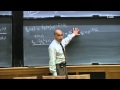
Understanding the Fundamentals of Quantum Mechanics: A Comprehensive Overview
Explore the core concepts of quantum mechanics, including wave functions, uncertainty, and energy levels in this in-depth guide.
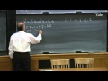
Understanding Quantum Mechanics: Wave Functions, Kinematics, and Dynamics
Explore the key concepts of quantum mechanics, focusing on wave functions, kinematics, and dynamics in a one-dimensional space.
Understanding Quantum Mechanics: A Comprehensive Guide
Explore the intriguing world of quantum mechanics, its principles, and the double slit experiment.
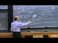
Understanding the Theory of Everything: A Deep Dive into Quantum Mechanics and the Schrödinger Equation
Explore the fundamentals of quantum mechanics and the Schrödinger equation, revealing the laws that govern how particles behave over time.
Understanding Quantum Mechanics: Wave Functions, Momentum, and Energy Discreteness
Explore quantum mechanics concepts like wave functions, time dependence, and energy quantization in an engaging manner.
Most Viewed Summaries

A Comprehensive Guide to Using Stable Diffusion Forge UI
Explore the Stable Diffusion Forge UI, customizable settings, models, and more to enhance your image generation experience.

Kolonyalismo at Imperyalismo: Ang Kasaysayan ng Pagsakop sa Pilipinas
Tuklasin ang kasaysayan ng kolonyalismo at imperyalismo sa Pilipinas sa pamamagitan ni Ferdinand Magellan.

Mastering Inpainting with Stable Diffusion: Fix Mistakes and Enhance Your Images
Learn to fix mistakes and enhance images with Stable Diffusion's inpainting features effectively.

Pamamaraan at Patakarang Kolonyal ng mga Espanyol sa Pilipinas
Tuklasin ang mga pamamaraan at patakaran ng mga Espanyol sa Pilipinas, at ang epekto nito sa mga Pilipino.

How to Install and Configure Forge: A New Stable Diffusion Web UI
Learn to install and configure the new Forge web UI for Stable Diffusion, with tips on models and settings.

If you found this summary useful, consider buying us a coffee. It would help us a lot!